Tweaking Antonacci's Simple Momentum Allocation System for 3× Market Returns

Revisiting an old classic with a new twist.

For those unaware, Gary Antonacci is a world renowned quant, most famously known for his best selling book and quantitative method: Dual Momentum Investing. In it, he describes a very simple, yet effective, asset allocation system that is based on momentum in the equity markets to outperform the market while minimizing turnover.

This bookcover is probably etched into your mind at this point, whether you’ve read it or not.

His breakthrough method hit the shelves in 2014. But, he has also authored many alternatives and updates to this type of asset allocation based on momentum.

I took one of his papers: Absolute Momentum: A Simple Rule-Based Strategy and Universal Trend-Following Overlay (SSRN Link here), reimplemented the algorithm in my portwine backtesting system (repo here), and found out that not only is the original paper still valid in today’s market, but a view simple modern day twists can exponentially improve the performance.

Demystifying Momentum Asset Allocation

Momentum based asset allocation systems are some of the simplest trading systems in the industry. They pretty much look at if an asset has momentum, and if so, allocates into it. There are other flavors in which out of a basket of 20 assets, you select the 3 with the most momentum or whatever. But, the rule set is pretty much always the same.

For the Absolute Momentum system, the rules are as follows:

1. For each asset, calculate the returns for the last 12 months.

2. For assets that return more than treasury bills over the last 12 months, invest in them.

3. For the others, rotate into treasury bills.

4. Every month, return to step 1 and repeat.

Ridiculously simple. And, Antonacci has the data to prove it.

But do these simple rules still apply today?

Replicating the Findings

I used my portwine backtesting system to create this simple strategy and run some simulations. However, from data back to 2000, and using the SHV ETF instead of investing in treasuries when out of the market, the news is not too amazing for Gary.

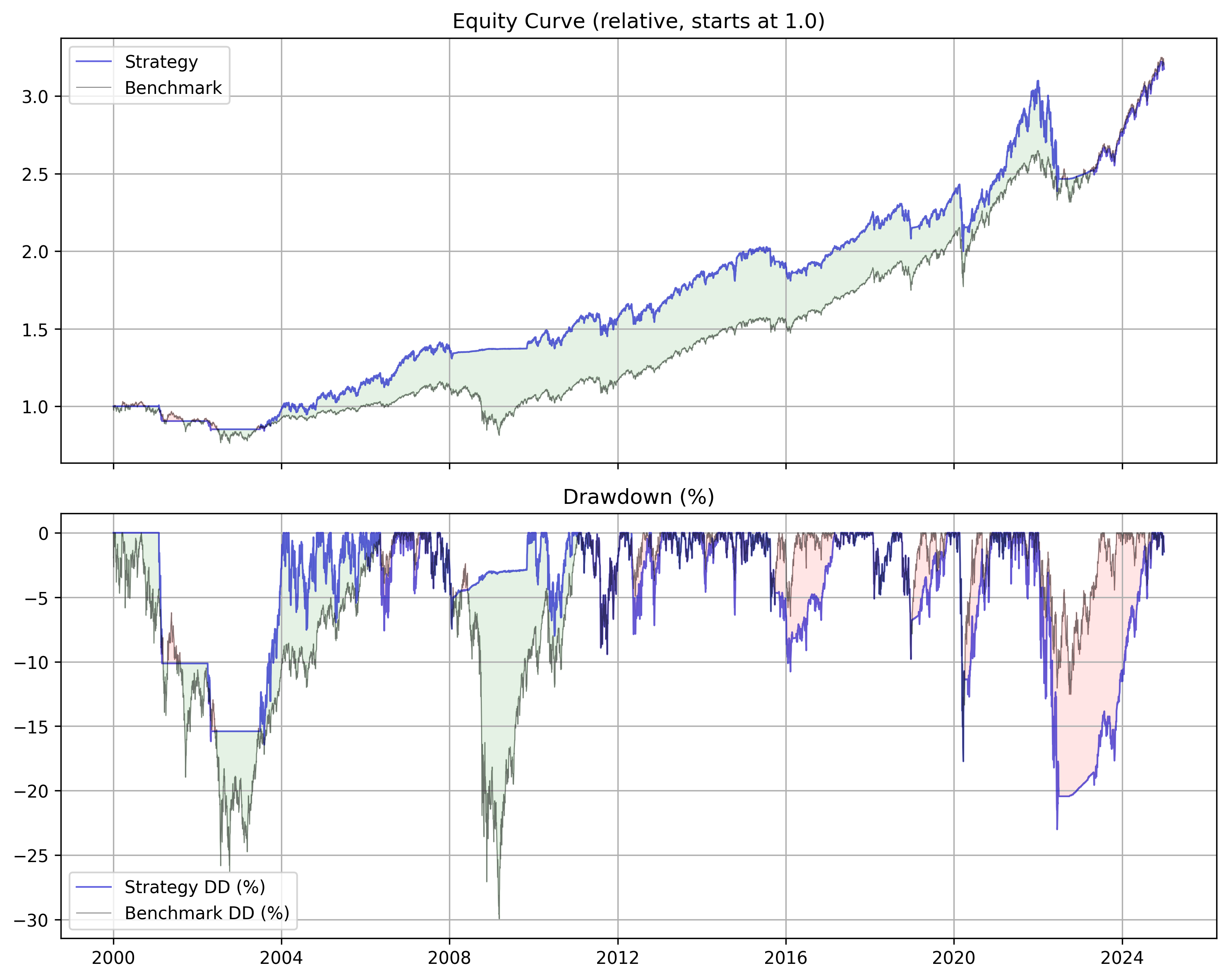
Absolute Momentum with SPY

---

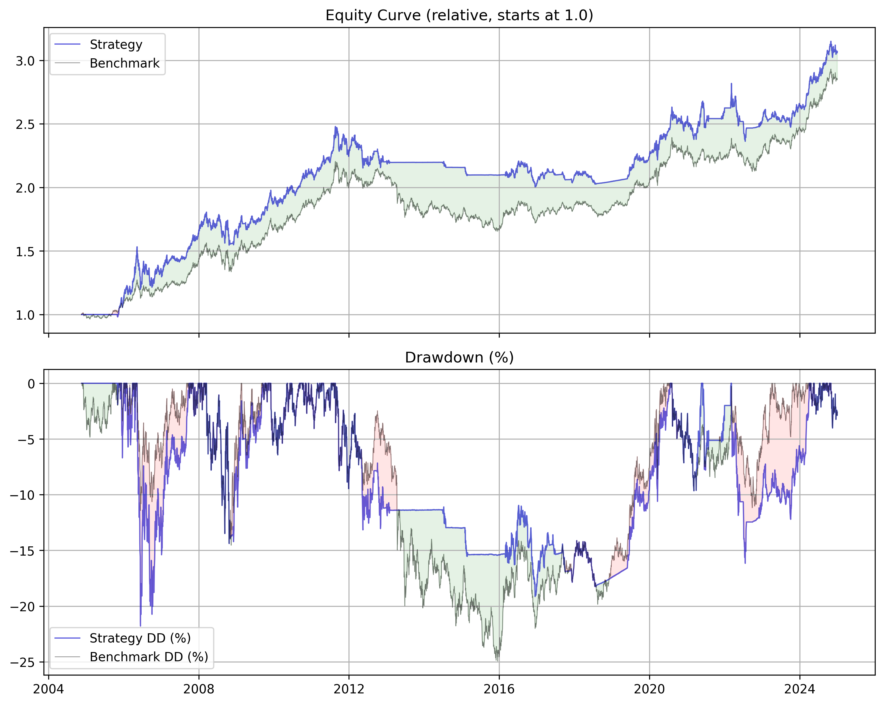
Absolute Momentum with GLD

---

Absolute Momentum with URTH (MSCI ETF)

---

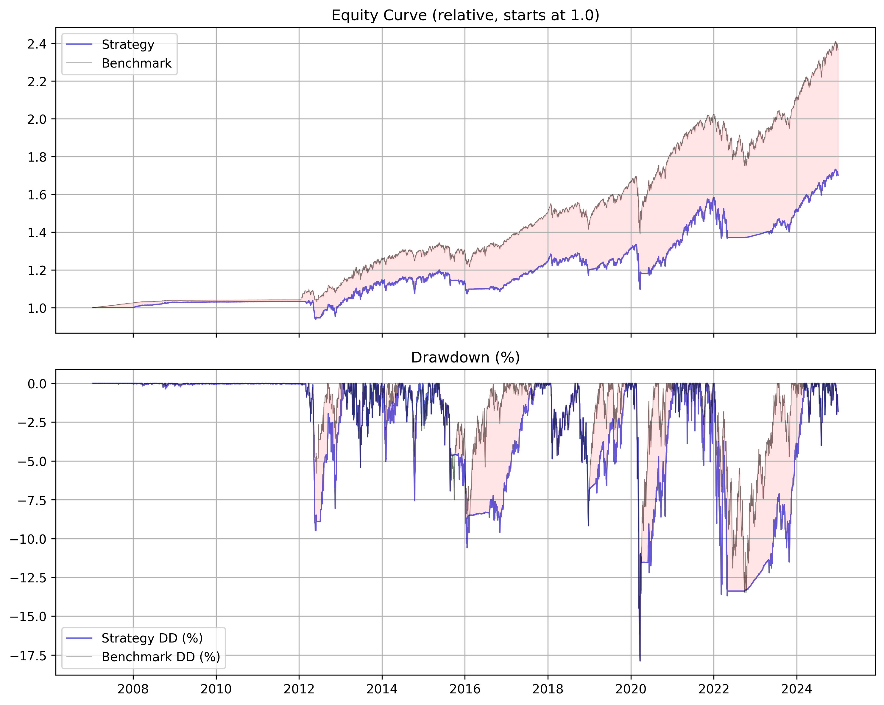
Gary’s system works well, especially with gold and assets where we sat out of the market in the 70s and 80s because treasuries were paying so much during those periods. When we start in 2000, when rates are low, sitting out of the market doesn’t really give us anything.

Even with the increased rates post COVID, we are not able to recover better performance than our MSCI analogue (URTH).

And Baskets?

But, what about a basket?

I tweaked the system to work with multiple assets such that we rebalance proportionally. If we hold 1 stock out of 10 in a basket, that 1 stock allocated 100% of the portfolio. If we hold 3 stocks out of the 10, each stock is allocated 33.3% of the portfolio. Etc.

I reused my Broad ETF basket from my first post:

broad_etfs = ["SPY", "QQQ", "IWM", "EFA", "EEM"] # No TLT or SHV
risk_free = "SHV" # TLT is another risk-free asset, won't include

Absolute Momentum with Broad ETF Basket

---

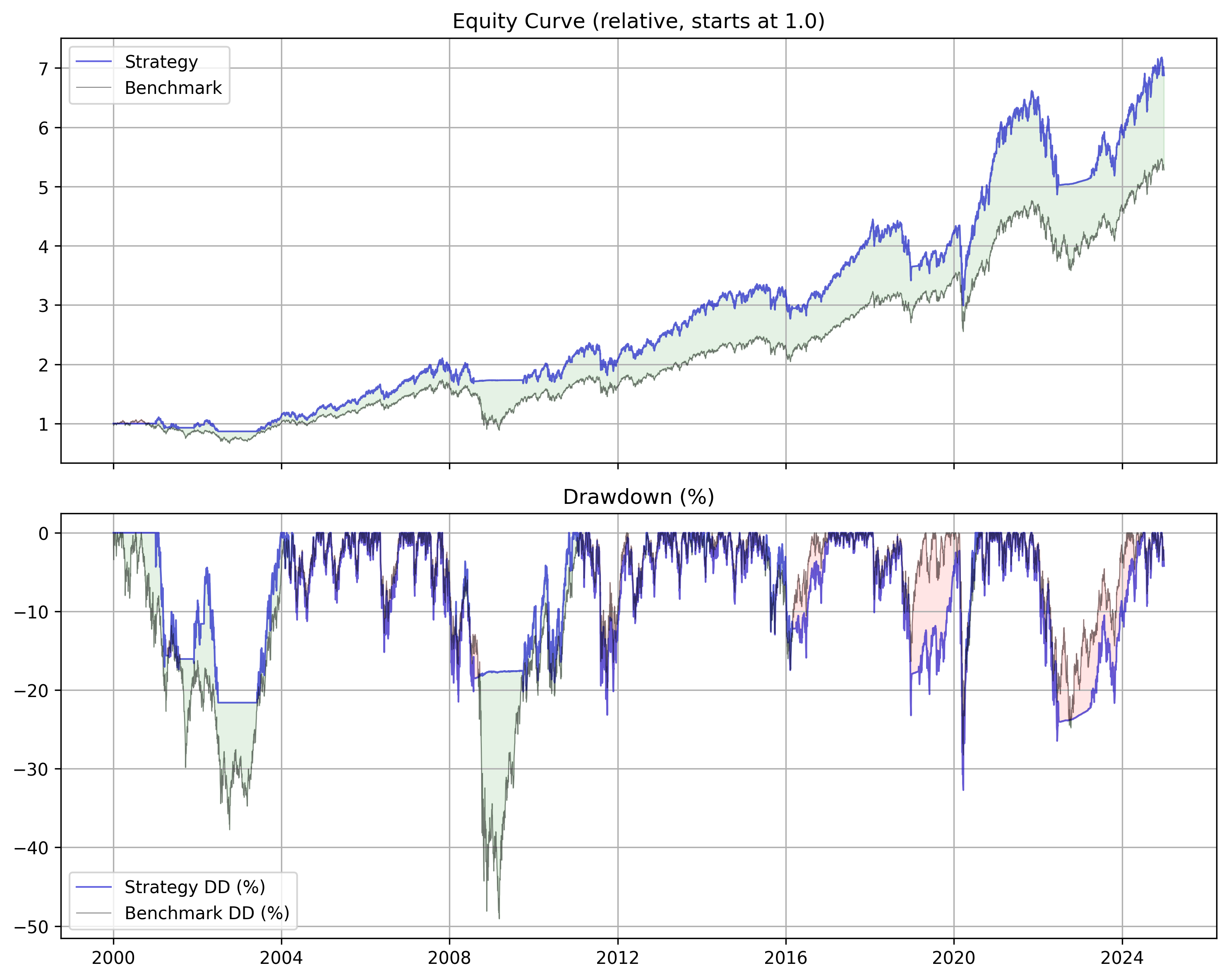
We cut off our drawdowns fantastically while outperforming an equally weighted. But, funny enough, post 2014 when most of his research is published, the system starts to decay against an equally weighted portfolio. Thus, while there is some validity to this strategy, I had to add some modern day tweaks to reignite the magic.

So, let us begin…

Innovation 1: Better Weight Allocation Methods

The original allocation method is binary: “Invest in the asset if the momentum is above 0, otherwise invest it in treasuries.”

This makes little sense once our basket sizes become huge. Out of 500 stocks, the variance in how much momentum surely has an effect on their forward returns.

I wanted to experiment with tweaking how much investment we put into each asset based on momentum, such as taking the top 5 ranked by momentum, scaling the weights proportionally based on how much momentum each asset has, etc. etc.

<PIC?>

Thus, I came up with several allocation methods to experiment with:

• equal: Equal weight among selected assets

• winner_take_all: All weight to highest momentum asset

• topk_equal: Equal weight among top k assets

• topk_proportional: Proportional weight among top k assets

• softmax: Temperature-scaled softmax weights

• power: Power-law scaling of weights

• threshold: Equal weight above quantile threshold

• rank_linear: Linear rank-based weights

• rank_exp: Exponential rank-based weights

• sigmoid: Sigmoid transformation of z-scores

• vol_adjusted: Volatility-adjusted weights

Applying the strategies to the original strategy and the NASDAQ 100

I applied the original strategy to the current NASDAQ 100 stocks and got this:

It’s nice. Edges out a little more than an equal weighted strategy. But here’s how it looks when we apply each strategy with reasonable default parameters.

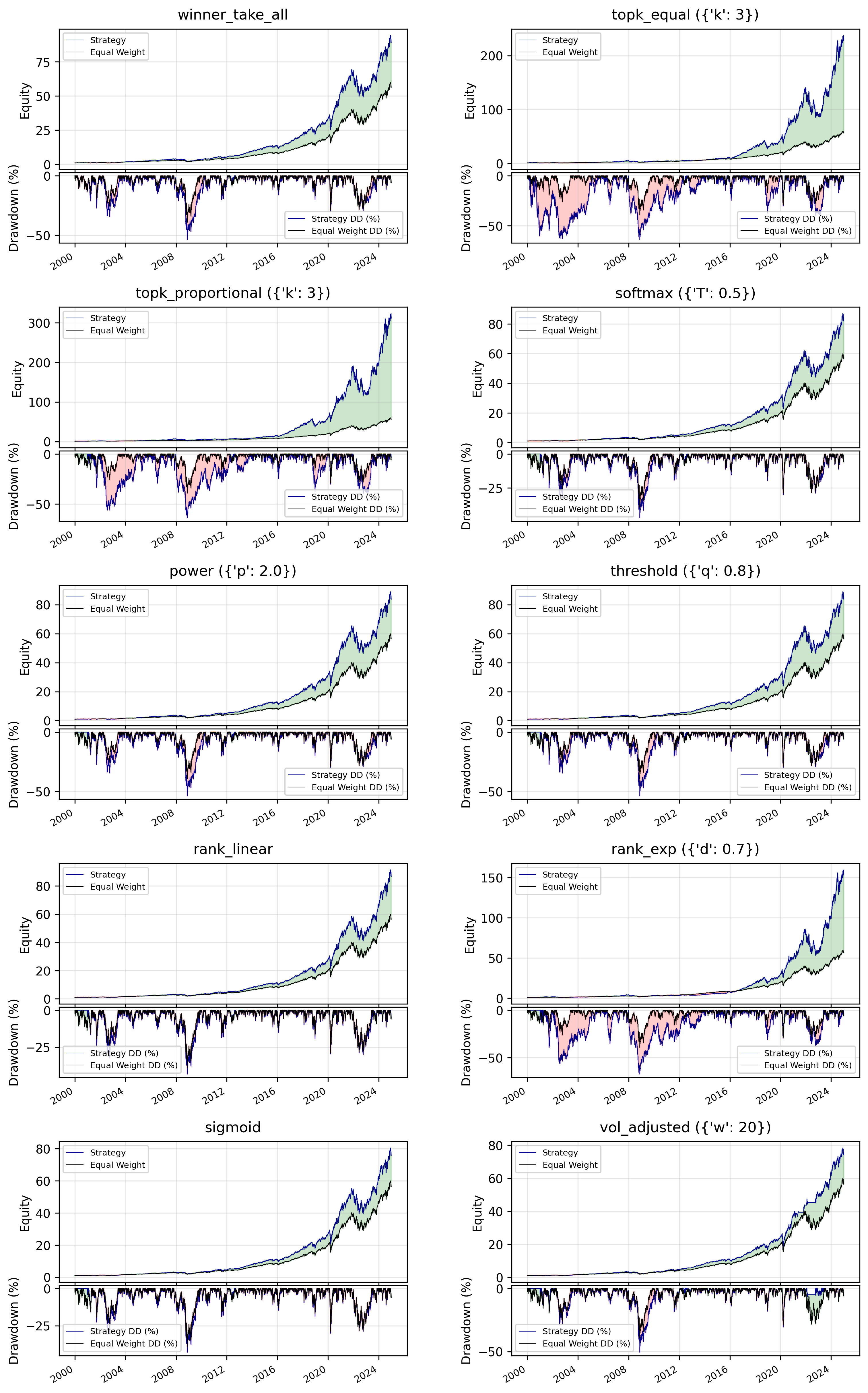
Right away, we see some of these strategies being clear ‘winners.’ The topk strategies really boost performance (at the expense of risk) and the vol_adjusted strategy avoids the recent Fed unwinding amazingly.

I’m particularly interested in topk_proportional which concentrates winners, yet adds a bit of diversification, limited with a proportional weighting feature which makes sure our diversification is based on which assets contribute the most momentum to the portfolio.

---

I then did a parameter sweep to see if changing the top k number made a difference:

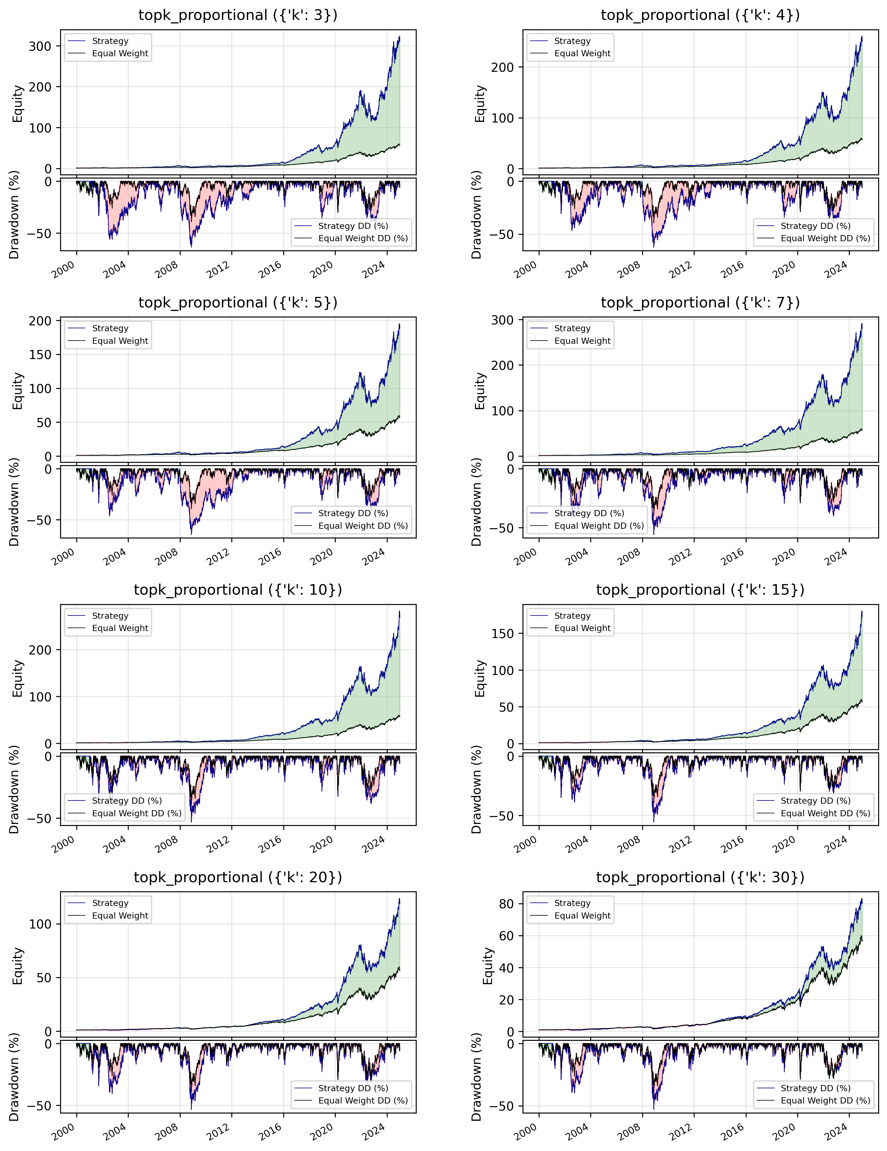
And our sweet spot seems to be between 7 and 10 assets, or the top 10% of the NASDAQ 100 at any point in time.

Innovation 2: Basket Selection With Genetic Algorithms

Next, I experimented with basket selection (which I have touched on in previous articles). Rather than using the hillclimbing algorithm that I used in the past, I used a genetic algorithm which just means I used the concepts of evolution to breed and mutate potential basket contenders until I found the best one.

This is particularly useful because picking a basket of 50 stocks out of 500 has 2,314,422,827,984,300,469,017,756,871,661,048,812,545,657,819,062,792,522,329,327,913,362,690 potential combinations.

Genetic algorithms help us navigate this complexity and arrive at ideal solutions more quickly.

Below is a cute video demonstration of genetic algorithms applied to solving the first level in Super Mario using neural networks. It’s worth a watch!

My system optimized for the Surefire Ratio, my own personal financial ratio which is far better than optimizing for Sharpe or total returns (you can read about here so you can implement it yourself).

Thus, I let the thing run for 200 generations and with 100 baskets in the population. I coded early stopping for when the validation set stopped improving along with the train set, with a patience of 25 generations.

For the allocation strategy, I used the topk_proportional with k set to 5. The basket was a selection of 50 stocks from the current SP500 components. The lookback time was kept at 12 months, but this can be experimented with.

The train period was set from 2000 → 2015. The validation set was from 2015 → 2020. The test was set from 2020 → now. Here are the metrics.

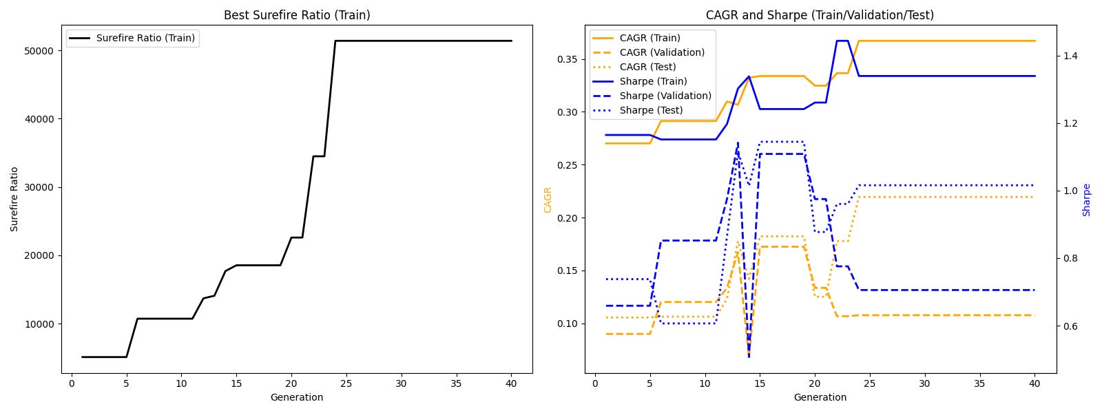
We see a clear evolution of success, although our population starts to ‘overfit’ to the train data after about 18 generations only.

The final basket from this run is the following, discovered at generation 15:

CMG, NFLX, WMB, TDG, UNH, CTSH, MSI, VST, TPR, BA, SW, NXPI, VTR, CHTR, LOW, VRSN, BWA, IR, V, VZ, AXP, GE, LHX, FANG, UBER, ACGL, TT, DLR, ON, AMP, CAG, NTAP, INVH, GOOGL, DPZ, DG, LMT, VICI, HBAN, COP, PODD, KIM, NVDA, SNPS, SPGI, CDNS, IEX, AZO, PARA, CBRE

The Findings

Thus, with these key innovations, I was able to take a classic system that was showing wear and tear and revitalize it into something much more modern and versatile.

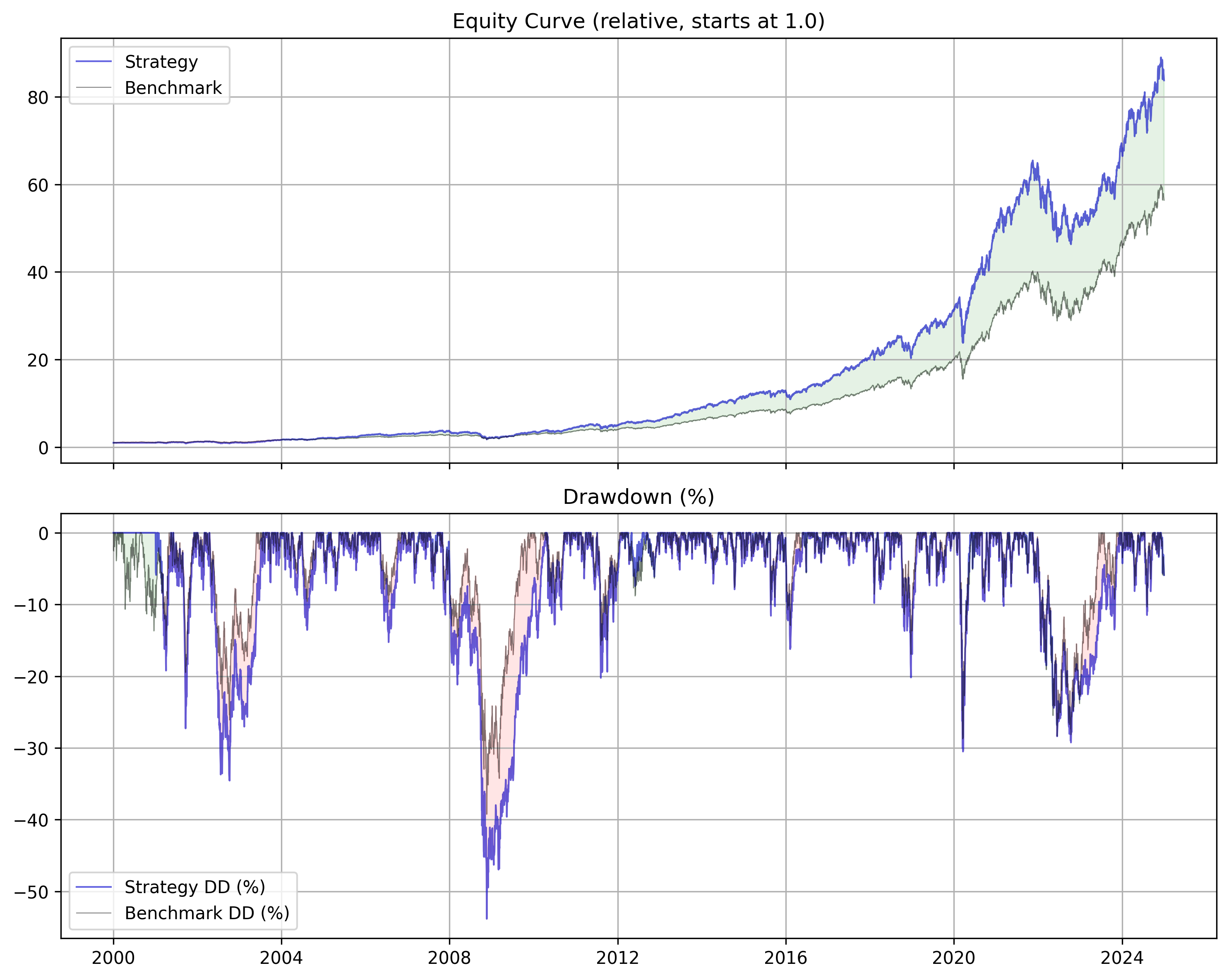
Strategy Performance

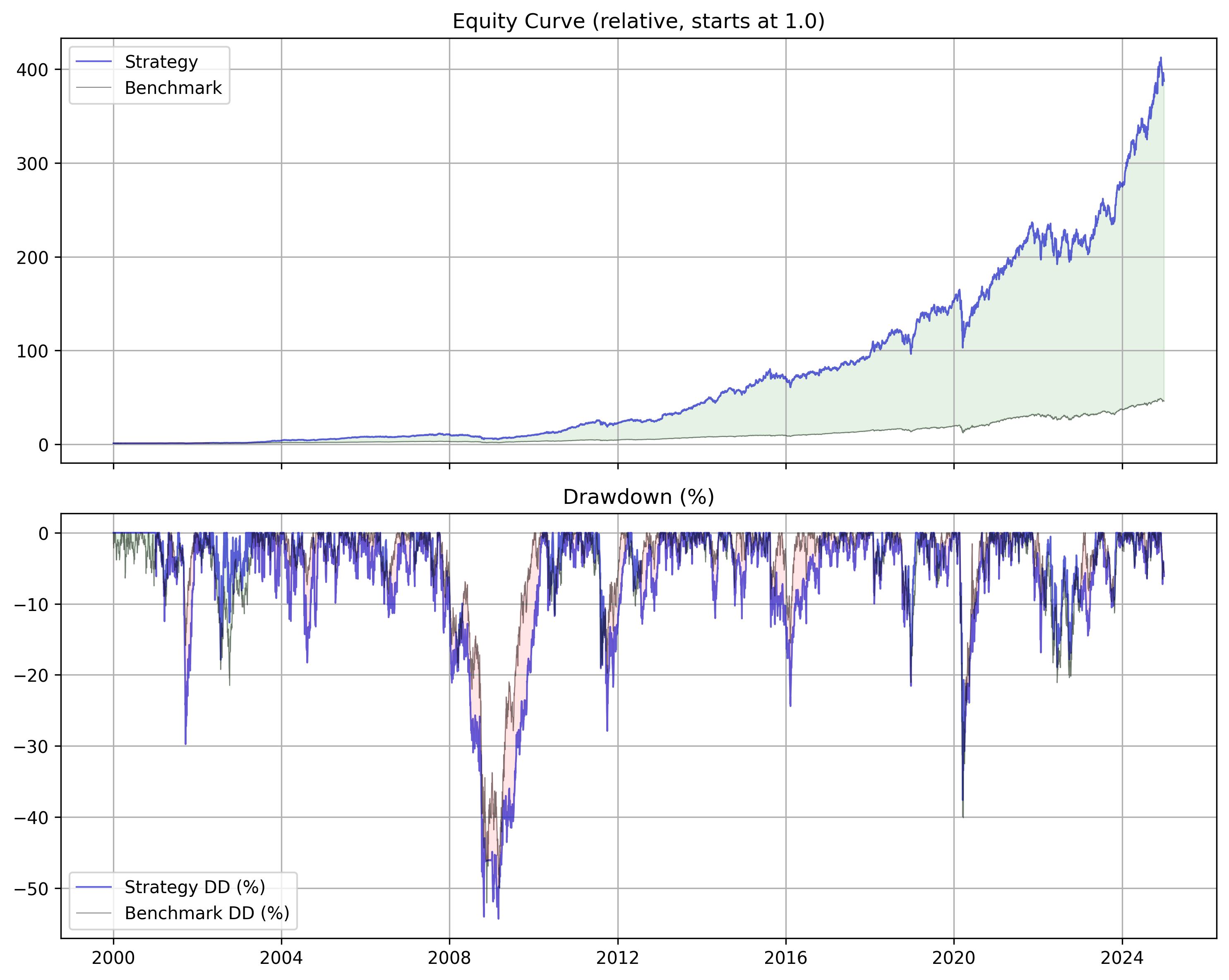
=== Strategy Summary ===
TotalReturn: 38638.47%
CAGR: 26.97%
AnnualVol: 22.98%
Sharpe: 1.17
MaxDrawdown: -54.32%

=== Benchmark Summary ===
TotalReturn: 4501.75%
CAGR: 16.58%
AnnualVol: 18.28%
Sharpe: 0.91
MaxDrawdown: -52.09%

=== Strategy vs. Benchmark (Percentage Difference) ===
TotalReturn: 758.30%
CAGR: 62.65%
AnnualVol: 25.71%
Sharpe: 29.38%
MaxDrawdown: -4.29%

---

Transaction Cost Analysis

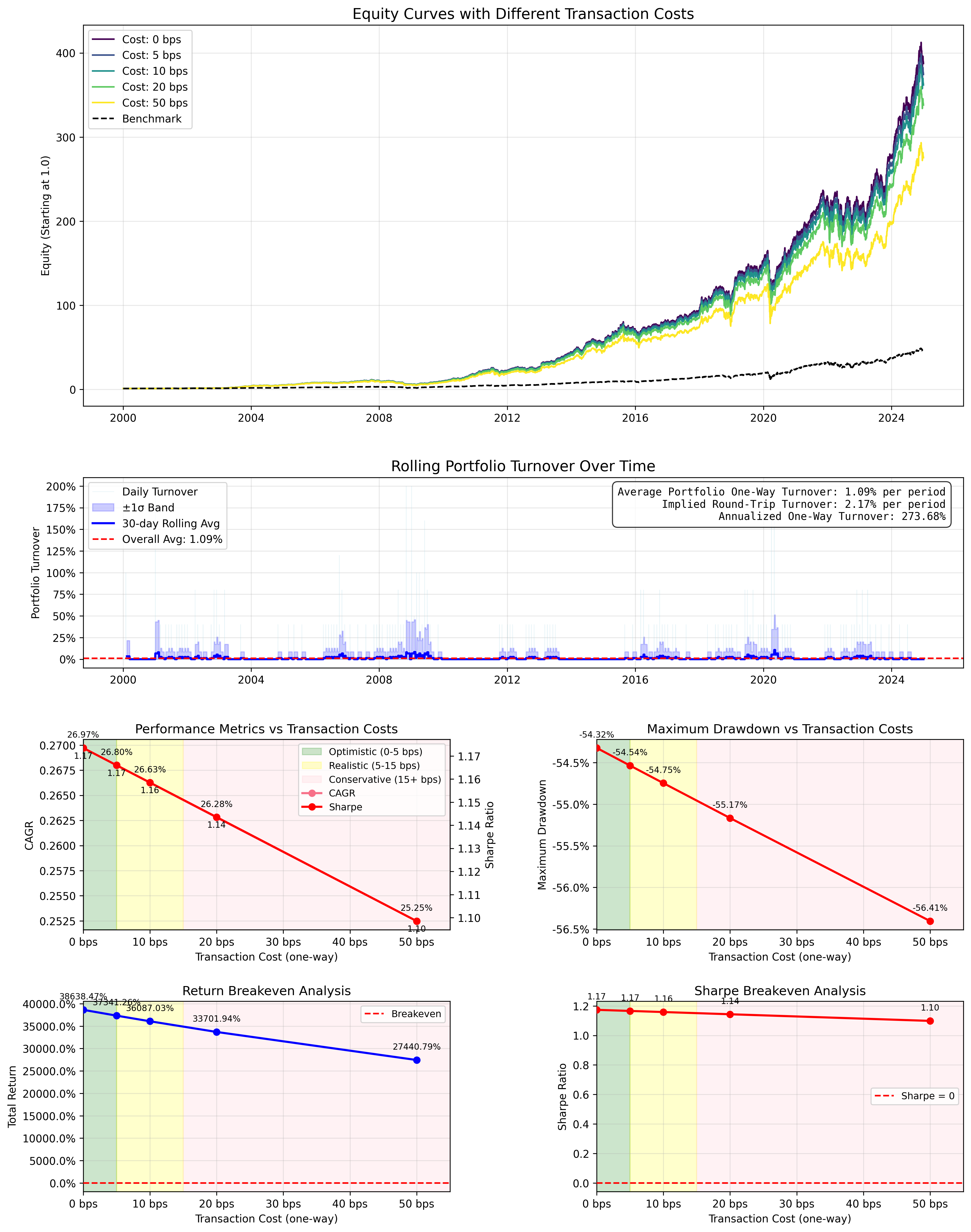
Due to the extremely low turn over (portfolio switches only once a month), the robustness is extreme. There is virtually no decay in the metrics even at 50 basis points.

---

Edge Decay Analysis

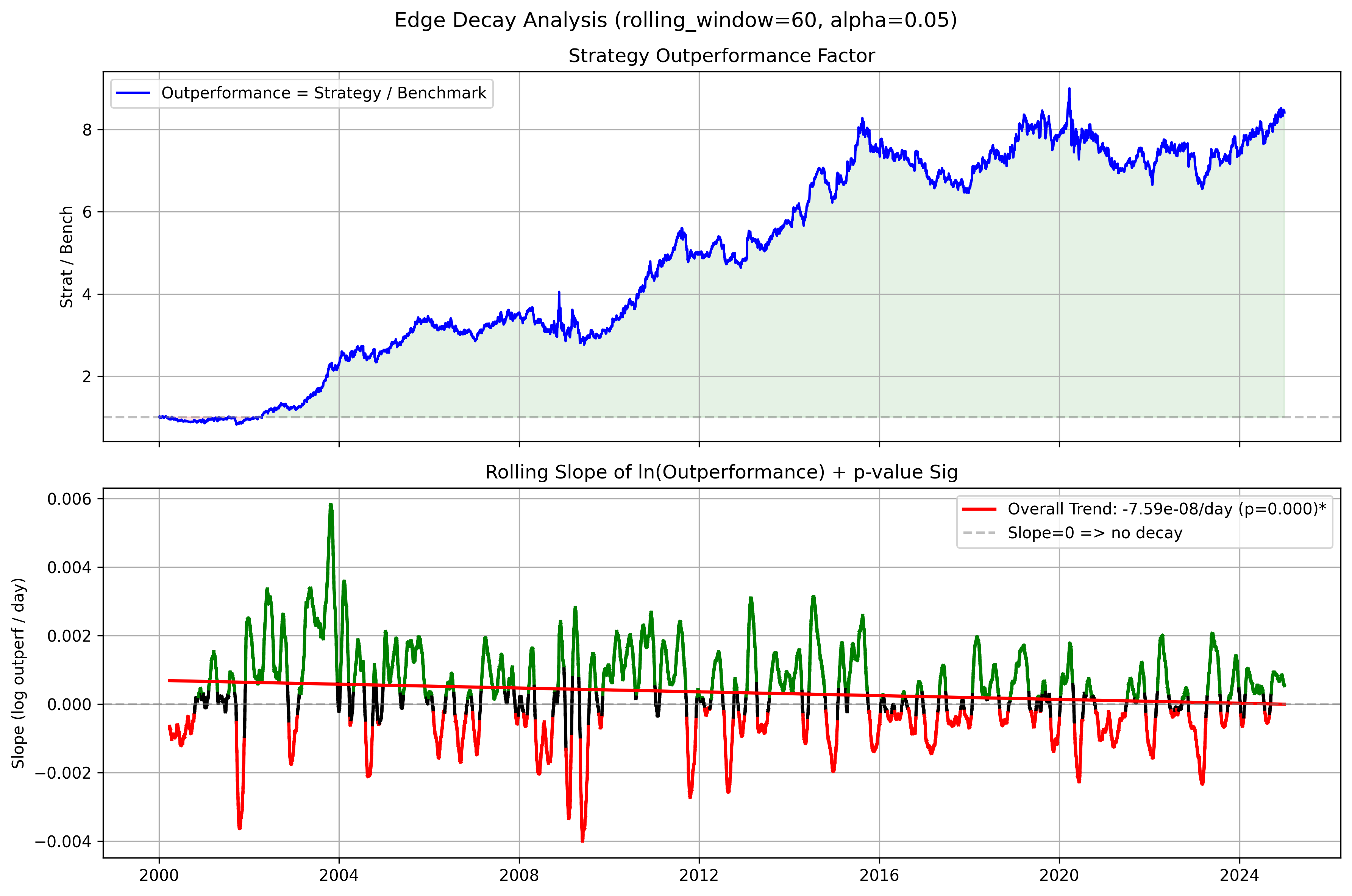
While the velocity of the edge seems to be decaying over time (2000 - 2008 had huge peaks of outperformance), the strategy still outperforms an equal weighted strategy.

Thus, we can carefully assume that our strategy still has some edge, although that edge is not as high as it used to be.

---

Overfit Analysis

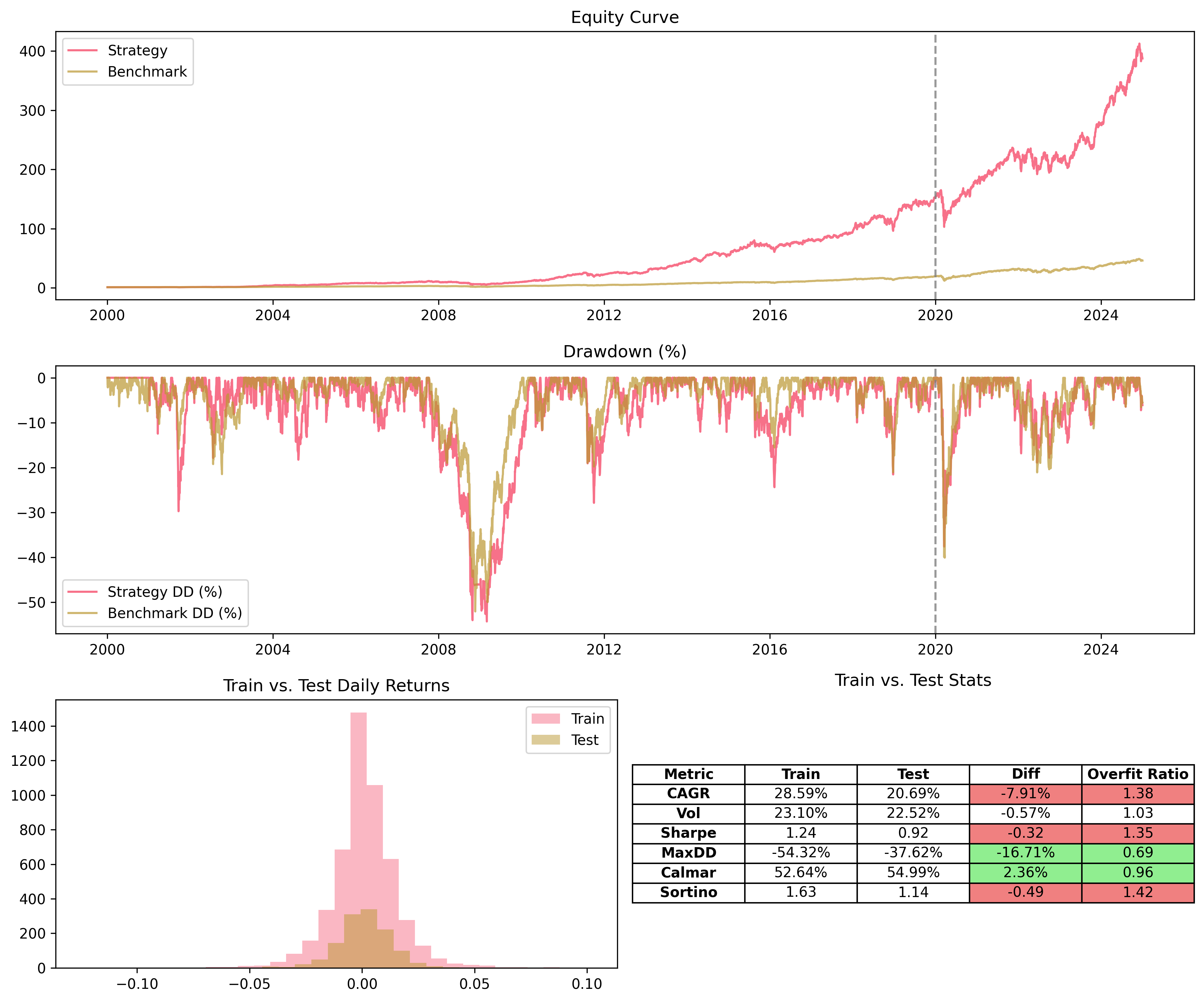
There is risk of overfit. This is probably due to the fact that our edge in the 2000s was higher than it is now. This is to be considered when taking this strategy live.

---

Doing it Yourself

Want to add these innovations to your own strategy development pipeline? Want to explore some more of Antonacci's systems and boost their performance?

You can download all the code to recreate these findings on the Paper to Profit Google Drive found here, including the vectorized strategy and genetic algorithm optimizer which you can use with any of your strategies!

If you do not have access, that is because you are not a paid member! Consider becoming a paid subscriber to gain access, but most importantly, supporting my research so I can continue doing what I love and bringing you great content.

If you want more of Antonacci's works, some are freely available on SSRN:

Optimal Momentum: A Global Cross Asset Approach

Risk Premia Harvesting Through Dual Momentum

A Century of Profitable Industry Trends

Thank you all for your support, and happy researching!