Testing Your Strategy for Robustness - Part 3 (Market Stress and Panic)

Simulating chaos and pain to give your strategy the final battle test.

Introduction

In the final part of the robustness series, I’ll dive into three methods you can use to battle-test your strategy by simulating pessimistic market dynamics. We all want to assume our strategy will be interacting with perfect fills and zero latency, but the reality is not so.

We will be executing in a fast-paced environment that is truly the survival of the fittest where all market places are out to take what they can take, and hopefully not from you.

That’s why it’s important to do what we can to protect ourselves by assuming the worst case scenarios. Specifically, I will be discussing:

1. Adding synthetic market noise to see if your strategy still holds up against messy data.

2. Adding transaction fees and finding the point of ruin for your strategy.

3. Isolating market regimes and determining what macro-market conditions are best for your system.

Our Example Strategy

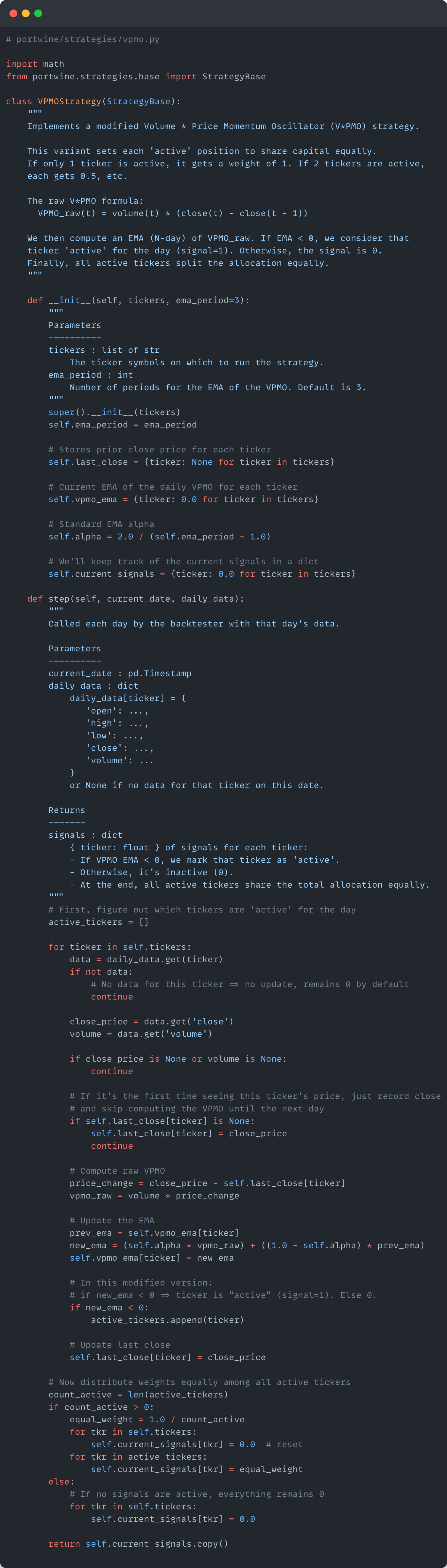
I built a very straight-forward Volume * Price Momentum Oscillator taken from The Encyclopedia Of Technical Market Indicators by Robert Colby that looks pretty good on paper. Here’s the strategy, written in my open-source backtesting framework portwine:

And here’s the resulting equity curve. Not too bad for a simple indicator based strategy!

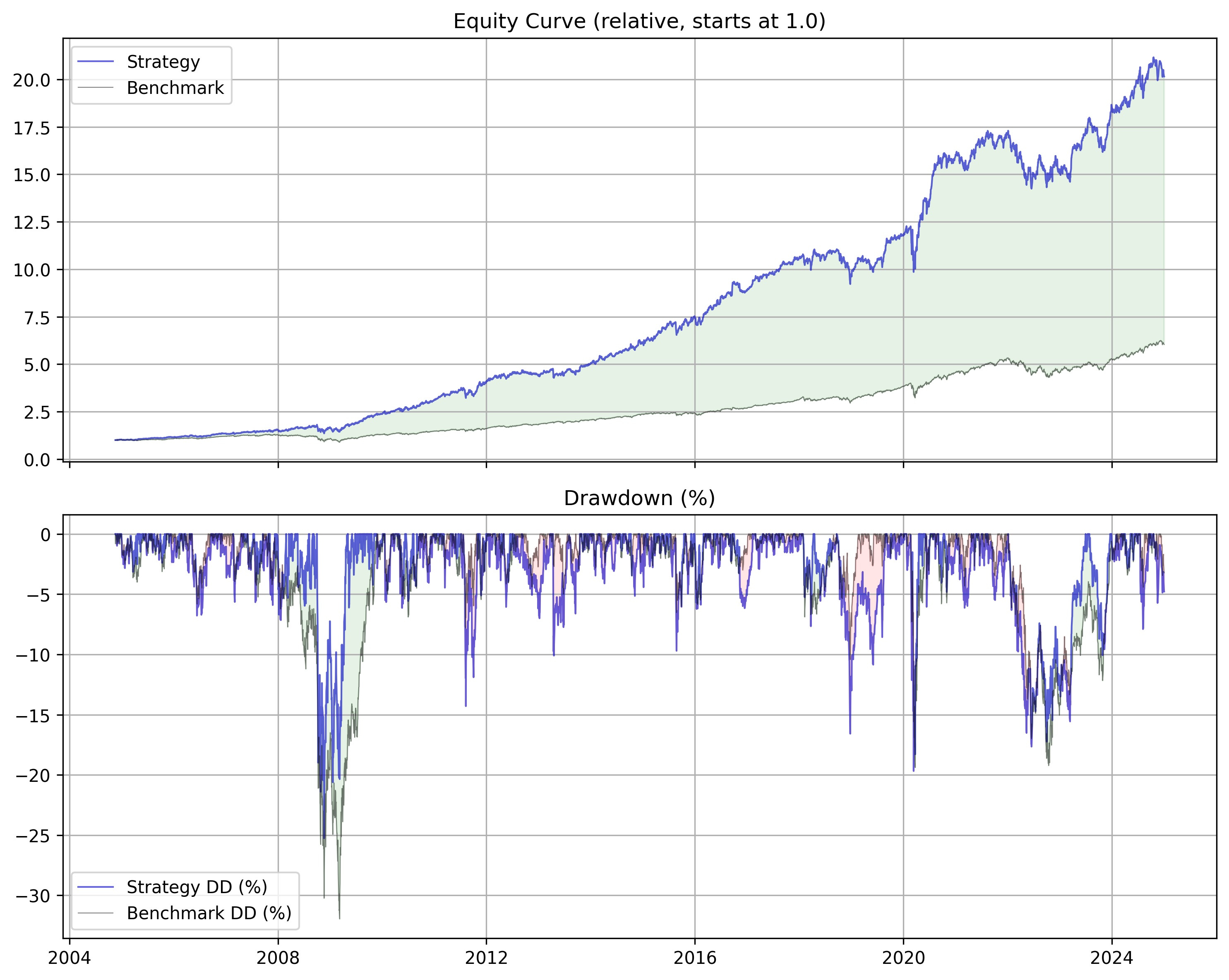
Ok, but how resilient is this thing? Will it collapse if the trades are executed at different prices? What about transaction costs? Does it hedge against market downturns during times of crisis?

Alright, one thing at a time. Let’s start with adding some noise to our prices to see if the strategy can still pick up the signal amongst the static.

Adding Market Noise

The goal here is to add an amount of noise to the price data that is enough to ‘shake things up’ but not too much to completely destroy the actual price action of the asset.

If our trading strategy has true alpha, it should be able to distinguish true signal from the noise. Thus, we can actually inject levels of noise into our price data that we use to backtest our strategies on to simulate what would happen with slightly different inputs.

I constructed a NoisyDataLoader object for my portwine backtesting framework (which is free and open-source here!) that injects an adjustable amount of noise based on rolling volatility of the asset. So, more noise added during more volatile periods, less during more calm periods. Here’s what that looks like:

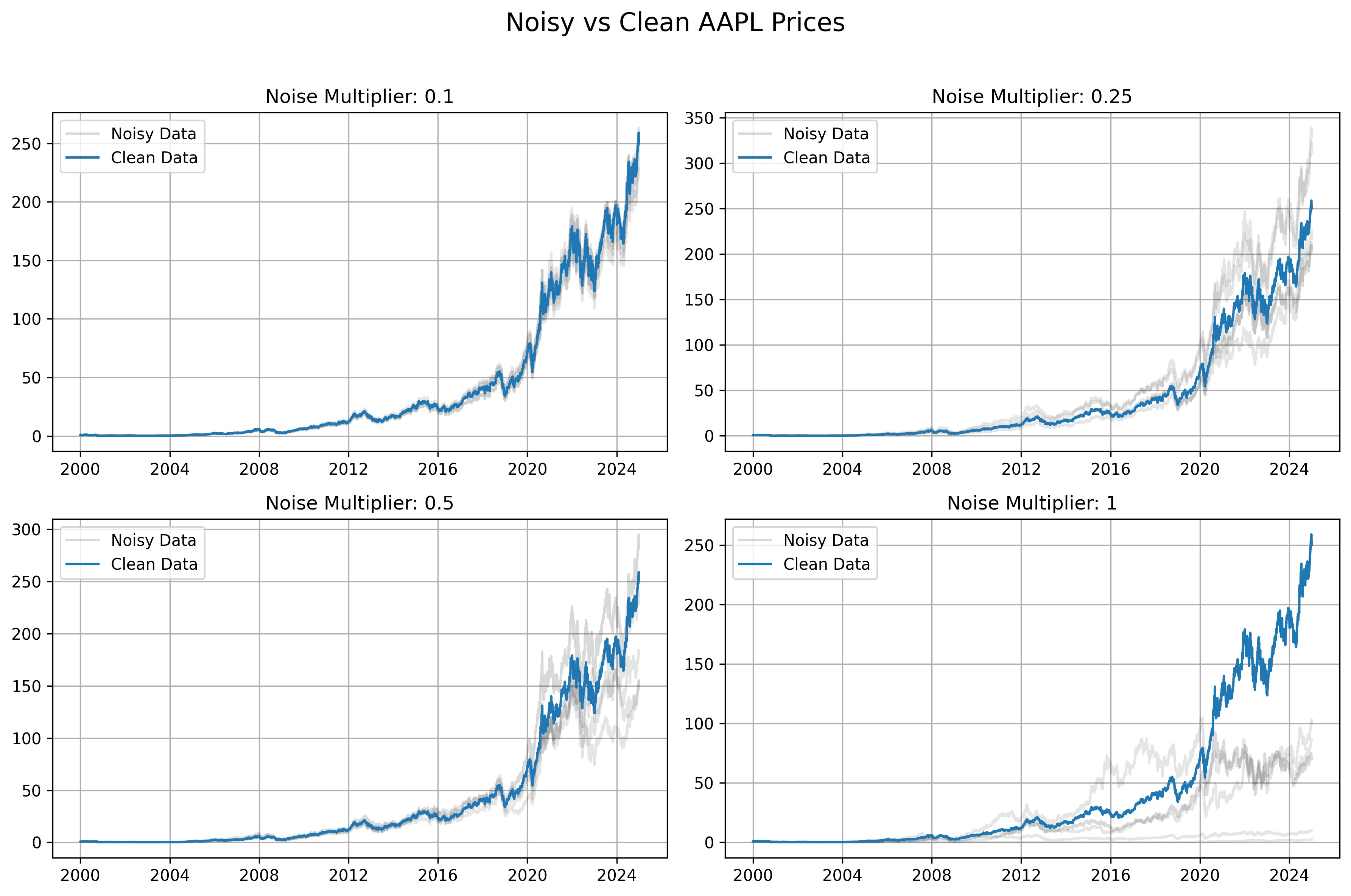
It’s not a perfect model of noise, but you can clearly see that as we increase the noise multiplier on the data loader, the paths really start to diverge from the original data. So now, what happens if we run our strategy against this noisy data?

I decided to run multiple iterations of each noise level to get a good average and then plot the decay in performance. As you can see, even a noise level of just 1 causes massive disruptions in the asset pricing. So, I decided to go with a list of the following levels: 0.05, 0.1, 0.15, 0.2, 0.3, 0.4, 0.5, 0.75, 1, 1.5, 2, and 3.

I then ran 100 backtests on each of these 12 noise levels for a total of 1200 backtests and produced this visualization:

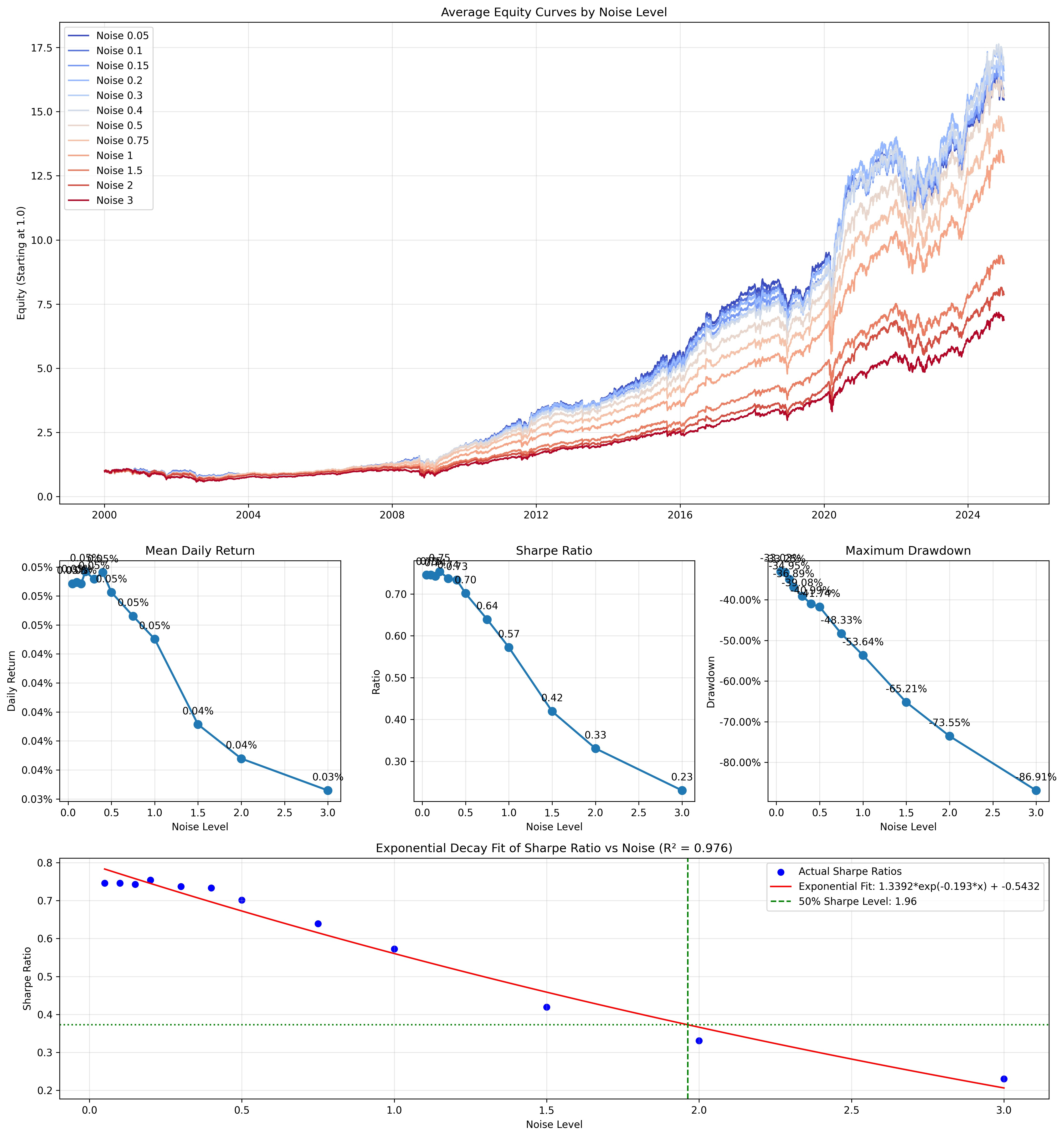
We can see a clear decay in all the tracked metrics: mean returns, sharpe, and drawdown. But, even at high noise levels, the strategy is still profitable. This shows robustness against bad pricing. The critical noise value is the point at which the Sharpe ratio is decayed by 50%. That being at 1.96 shows that our strategy is very robust against noise.

Transaction Cost Modeling

Let’s move on to something a bit more usual: transaction costs. We all want to assume that trading is free, and in some cases with commission-free trading, it is. But this is not a good assumption to make. Transaction cost modeling gets us even closer to reality as to what our backtest says, and what we will actually experience in the real world. Even if you can get your commissions close to zero, you will still be hit with potential spreads, slippage, and regulatory fees that you simply can’t avoid.

Typical one-way transaction costs (each side of the trade) can be assumed as the following based on asset class:

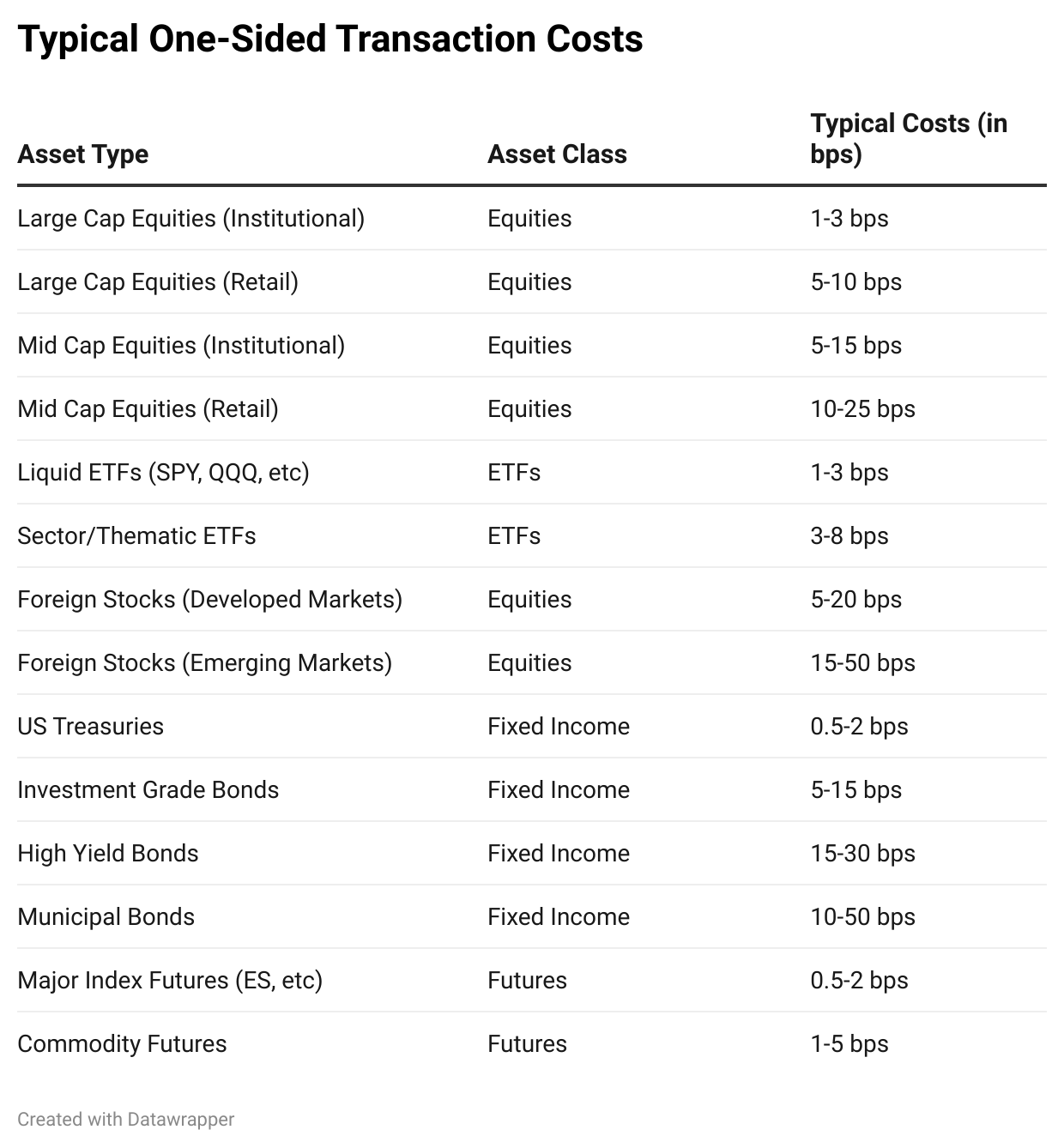
With that in mind, we now have to model our transaction costs. We do this by taking the weights from our backtest and determining the change over time. If we were in the market 50% SPY and 50% GLD and tomorrow we will be 60% SPY and 40% GLD, then our turnover and transaction costs are only applied to the 10% of the portfolio that bought more SPY and the 10% of portfolio that sold the GLD to do so. Thus, our transaction costs would be only 20% of our assumption (let’s say 2 bps because we’re trading liquid ETFs in this example). So, 20% of 2 bps is 0.4 bps of fees applied on that day.

So, when we model the cost of 2 bps, we are applying that to the turnover of assets. I went ahead and modeled the costs from 0 bps → 24 bps to give a wide range of outcomes to asset:

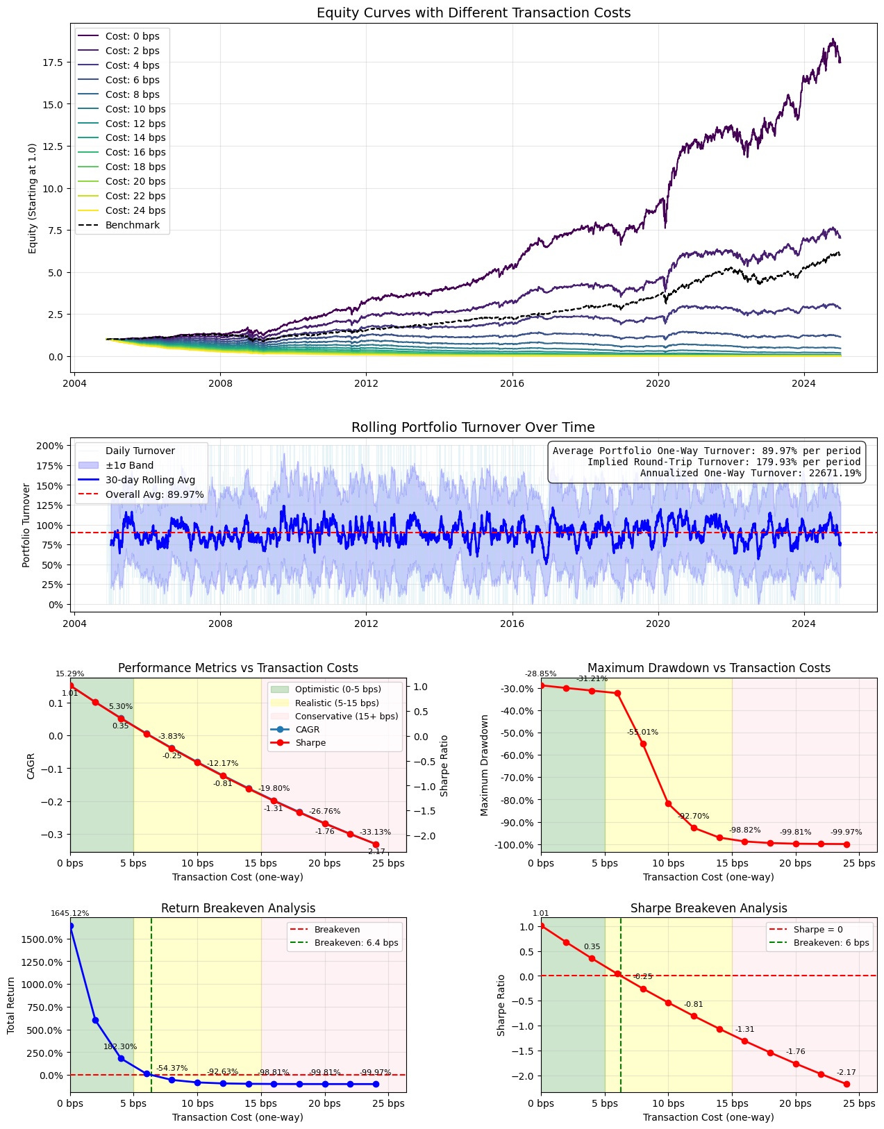
The turnover for this strategy is very high. That’s not too surprising because it acts more as a ‘signal’ strategy than a portfolio allocation strategy. Trades are either in or out based on the VPMO indicator. In fact, the rolling turnover sits at right below 100% which means that every day we are pretty much buying and selling the total portfolio’s value. This in turn costs us a lot in transaction costs, which you can see in on the main equity curve and in the breakeven analyses below.

The strategy has a complete breakdown at anything below 6 bps which is very bad. Even just 1 bps of fees takes the strategy from 1645% returns to about 600% returns. That level of sensitivity to fees makes me very insecure about actually deploying this live. Market conditions are usually working against us and if I take a -62.5% decay in my strategy due to a single basis point in fees… well then I’m probably dead in the water before even launching this thing.

Note that this strategy can be robust in a noisy environment and brittle against transaction fees because noise moves in both directions. It can either aid or hurt us, and generally the noise test will add noise in both directions evenly. Transaction costs only move against our P&L.

Regime Change Analysis

Lastly, we want to see how this strategy performs under different regimes. A regime is described as some sort of market that exhibits unique characteristics for a certain set of time. For example, a bull market versus a bear market. These are regimes. A sideways market, or a high volatility but no directional change, are also types of regimes.

I define 7 regimes here to analyze:

1. Strong Bull - Heavy positive trend, normal volatility

2. Bull - Positive trend, normal volatility

3. Sideways - Low trend, low volatility

4. Bear - Negative trend, normal volatility

5. Strong Bear - Heavy negative trend, normal volatility

6. Volatility Up - Upward bias, high volatility

7. Volatility Down - Downward bias, high volatility

These 7 types of regimes describe pretty much every market scenario that we can find ourselves in. We then can identify the benchmark’s regime (SPY in this case) and take all moments from each regime to compare the benchmark against the strategy.

For example, let’s take very day that the SPY is in a bear market and accumulate all the returns from the benchmark and strategy together to see how both perform comparatively. Here’s how that looks:

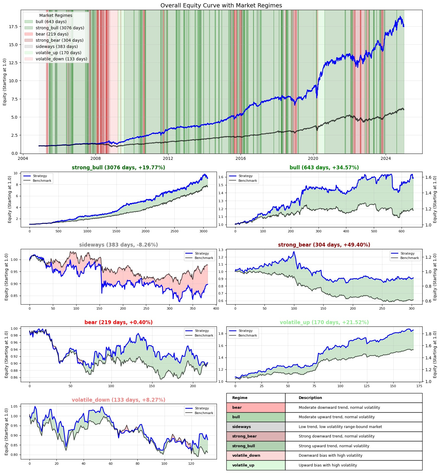
In most cases, the strategy is outperforming the benchmark (assuming no transaction fees), which is a good thing. There are some regimes like the sideways market and volatility down market where it struggles. But all in all, it shows good results. The sideways market struggling makes sense because this strategy uses basically an EMA filter to identify trends. So if the market is not ranging, a ton of false signals are going to be generated.

We can use this information to potentially add some sort of range filters to help us filter out sideways markets and ‘bad times’ for the strategy.

The Verdict

So what’s the end verdict for this strategy?

1. It is robust against noise. I have no reservations against the quality of the underlying signal being generated. ✅✅

2. It is highly sensitive to transaction costs. The impact that even 1 bps has on this strategy is so detrimental, that it invalidates it right here. ❌❌❌

3. It does pretty well in most regimes, but struggles in sideways markets. The outperformance in the other regimes makes the sideways market underperformance is fine. But, it would make sense to investigate a sideways market filter to increase performance. ✅

At the end of the day? Do not deploy this strategy. It is a loser based on transaction fees alone.

The equity curve looked great thought, didn’t it? It’s sad that we have to let this one go. But, it’s better to let it go now before it robs us of our money and our hopes and dreams live in the market.

---