Testing Your Strategy for Robustness - Part 2 (Fighting Overfit)

How to defeat the demon of our scariest nightmares.

In part 1 of this series, we talked about basic statistics that you can use to prove your system has an edge. But we didn’t get into the scariest threat of them all: overfit.

For those who have not met this beast, be thankful. Overfitting is when you tune the parameters of your trading strategy to optimize for returns, only to have it completely fall apart when you test it on new data. It’s a complex problem of optimization, but only optimizing ‘enough’ to avoid overfit. Luckily, you have me as your savior to guide you through the jungle.

My face when realizing that my 3 Sharpe Ratio, 200% CAGR strategy actually is just overfit and returns -3% CAGR out-of-sample

How many of us have encountered an amazing equity curve, only to have our dreams smashed once we realize that it’s simply overfit or has lookahead bias? I think everyone of us have run a backtest that looks like our ticket to paradise and are already spending the money in our heads before we realize that we forgot to shift our signals and we’re looking at the current days close to calculate signals at the open.

Not only is this experience demoralizing, it can waste our time going down rabbit holes that do not yield good results. Therefore, it’s important to know how to protect ourselves against this monster so we can minimize our pain, and maximize our success.

There are several causes of overfit that we must address:

1. Lookahead bias / data snooping

2. Survivorship bias

3. Model complexity

In this article, I will go through these concepts, but more importantly what you can do about them in your own research.

Lookahead Bias & Data Snooping

The basic concept of lookahead bias and data snooping is that we inadvertantly expose our trading strategy to something that is happening in today to points in the past which is not possible without time travel.

We all know about calculating some indicator, and then taking action on that same day, only to forget that we cannot use the close price of a candle to calculate a moving average and take an entry on the open. There’s no way to know the closing price at the open of the same candle.

For example, one of the most common screwups is shuffling your training and test data if you’re using something like SciKit-Learn’s train_test_split method. This method shuffles data on default, so unless you set it to False, it will happen. Shuffling is great for data that is not time contingent. But, when we do this for financial data, we bleed all of the future into the model and it instantly becomes invalid.

However, there are other more subtle versions of lookahead bias and data snooping that we need to be aware of. Specifically, when calculating features and signals.

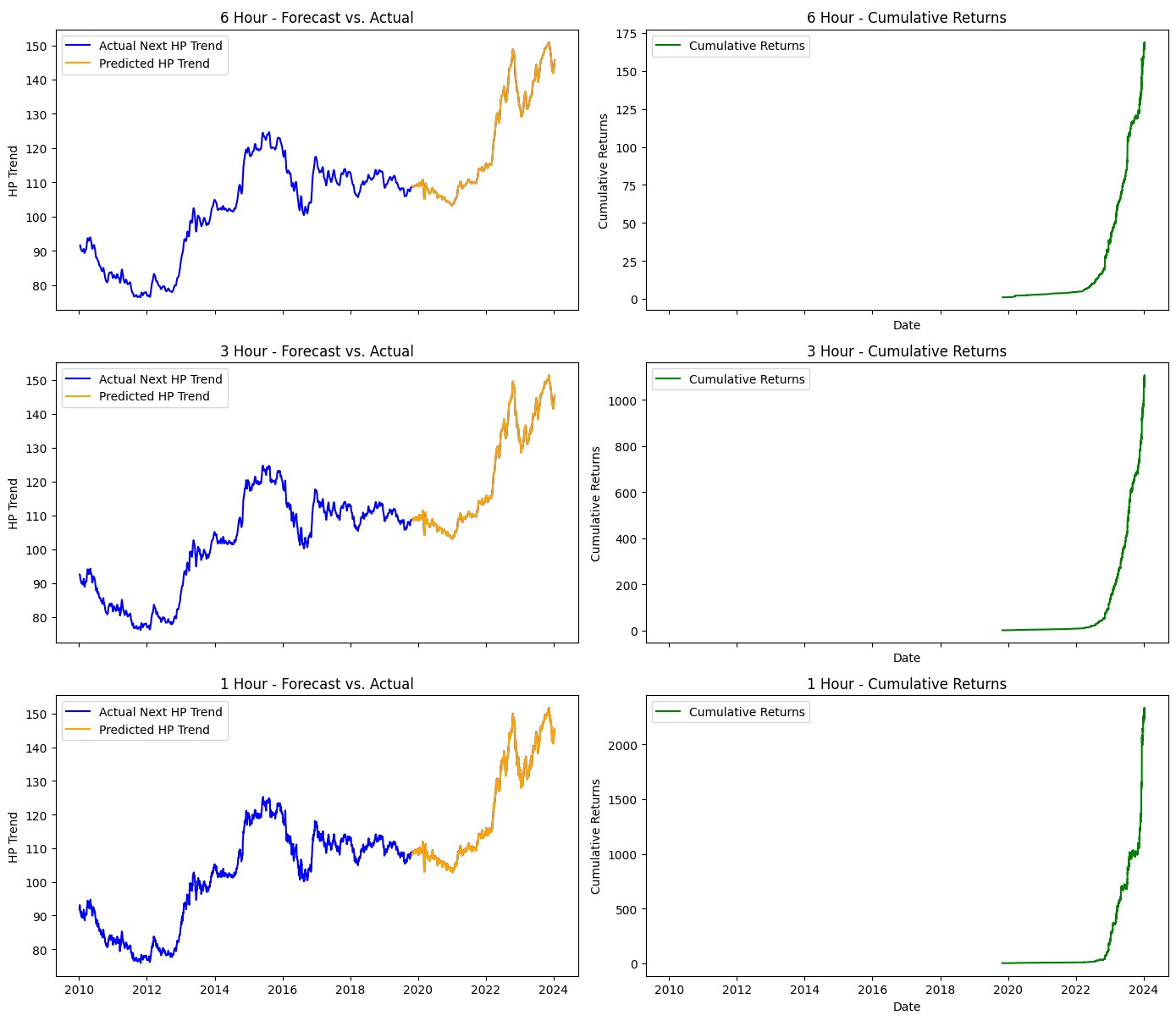
I was implementing a strategy that I had read in a research paper that used a Hodrick-Prescott filter to smooth out FX data to come up with a trend signal. The paper laid out the method and the impressive equity curve so I recreated it and did the same. Above are my results. On a 6 hour system, the strategy made 17500% over four years. 3 hours? 10000%. 1 hour? Over 20000%. I was rich.

Incredible! And all my features were lagged and my target was shifted forward, look!

def generate_features(data, hp_trend, hybrid_trend, loess_trend):
    """
    Build a feature DataFrame:
      - hp_trend, hybrid_trend, loess_trend, raw_return,
      plus one-period lags of each.
    Target is the hp_trend one period ahead.
    """
    df = pd.DataFrame({
        'hp_trend': hp_trend,
        'hybrid_trend': hybrid_trend,
        'loess_trend': loess_trend,
        'raw_return': np.log(data / data.shift(1))
    })
    df['hp_trend_lag1'] = df['hp_trend'].shift(1)
    df['hybrid_trend_lag1'] = df['hybrid_trend'].shift(1)
    df['loess_trend_lag1'] = df['loess_trend'].shift(1)
    df['raw_return_lag1'] = df['raw_return'].shift(1)
    df['target'] = df['hp_trend'].shift(-1)
    return df.dropna()

So, on paper, it looked like I was a millionaire a thousand times over. But what I failed to understand, and what the paper failed to carefully disclose (until I went back and read it more carefully of course), is that the Hodrick-Prescott filter is not a causal filter. I, of course, at the time was not aware of this fact. A non-causal filter is a filter that passes over the entire dataset to then create it’s filter. In this algorithm’s case, it does that to calculate historical cycles and trends. So, it has to have the full set of data to be able to do that.

Furthermore, the Hodrick-Prescott filter is used mostly for things like economic modeling and business cycles where you can expect cyclicality to hold up over time. This is not really the case with intraday FX. Rereading the paper confirmed this for me as it was one of those ‘theoretical papers’ that was just ‘showing the descriptive potential’ of the filter and not trying to allude that it was a source of alpha. Whatever.

So, instead, I decided to recode the system and calculate the Hodrick-Prescott filter at every time step using all the history I knew up to that point to calculate the next point forward. I figured that this should work, or at least work after an adequate amount of historical data was fed into the filter.

Unfortunately I was wrong.

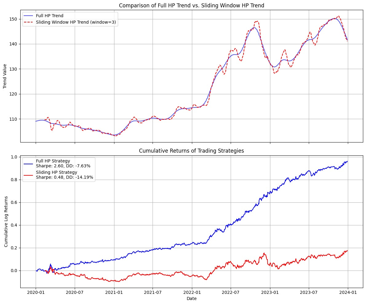
The blue line shows my hopes and the red shows my stagnating reality. There’s a Matrix reference in there somewhere.

Thus, lookahead bias and data snooping is not just about ‘am I using the current close to calculate something at the current open?’ You also have to understand deeply the methods that you are using and taking advantage of to avoid these pitfalls.

Survivorship Bias

Another source of overfit we need to be aware of is the survivorship bias.

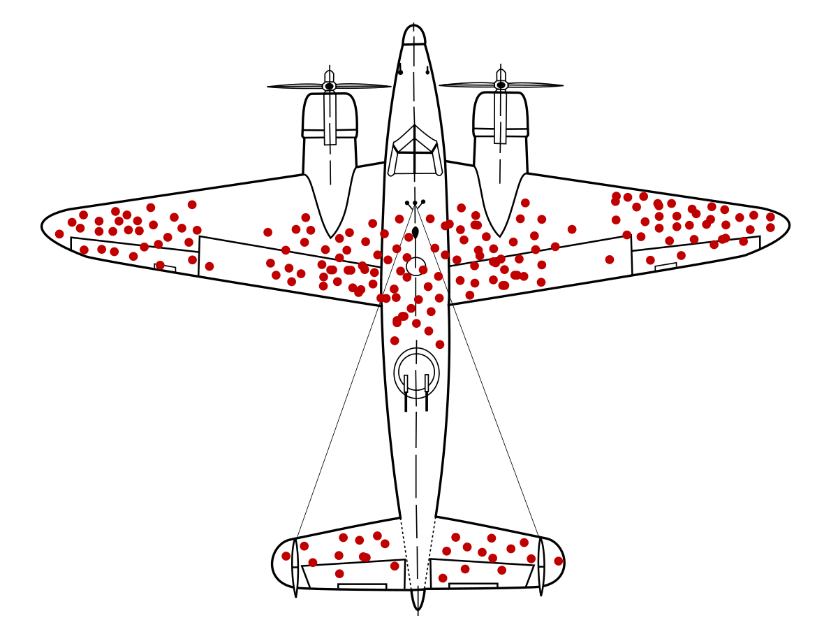
Surely we’ve all seen this plane before. It’s from a famous study from World War II where statistician Abraham Wald working with officials to try to figure out how to reinforce their fighter jets. The naive assumption was to reinforce the points that had the most bullet holes in them statistically.

But what Wald ingeniously pointed out is that ‘we aren’t considering the planes that never made it back and for those we have no data on.’ Curiously, there were no bullet holes in very specific parts of the planes (seen above). And so, what that meant really was the weak points were in those areas where we had no data because those planes were shot, crashed, and never made it home.

Similarly, when we look at our universe of data, we look at the 'blue-chip’ stocks and make the foolish assumption that we knew they were going to be ‘blue-chip’ stocks since they IPO’d. Amazon during the 2000 Dot Com crash fell 93% and stayed below it’s previous all-time-high for 7 years. What asset manager, after taking a 93% loss, is going to hold onto a stock which what was part of essentially a crypto bubble at a time.

What’s the best trading strategy? Invest in Apple. Or have been invested in Apple since the IPO. But how many people pulled that off?

Furthermore, how many companies would your strategy would have traded if you ran it back in 2000 that no longer exist? How many companies are completely defunct?

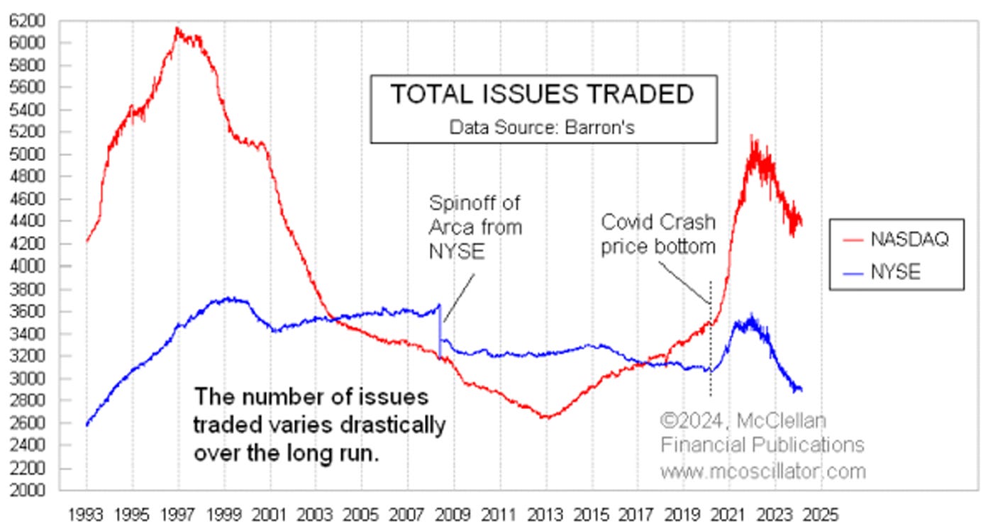
In fact, until COVID when we saw a ton of SPACs and IPOs emerging, the number of traded companies on the NASDAQ was in deep decline, over half the size of what it was at its peak.

Thus, when developing strategies, especially ones that trade stocks, it is important to benchmark your strategy against something that makes sense or use assets like ETFs that are rotating assets and do not have survivorship bias (no ETF knew Apple was going to skyrocket before anyone else, as they generally follow simple rules and guidelines).

If your strategy trades stocks that in recent history have been hot, like Apple, Amazon, and Tesla, compare your strategy not against the SP500, but against an equally weighted portfolio of itself. This will show you the true edge that your strategy has against simply being in the right place at the right time.

Model Complexity

Let’s assume you have a model that you are optimizing the parameters for. I have a mock strategy below to demonstrate.

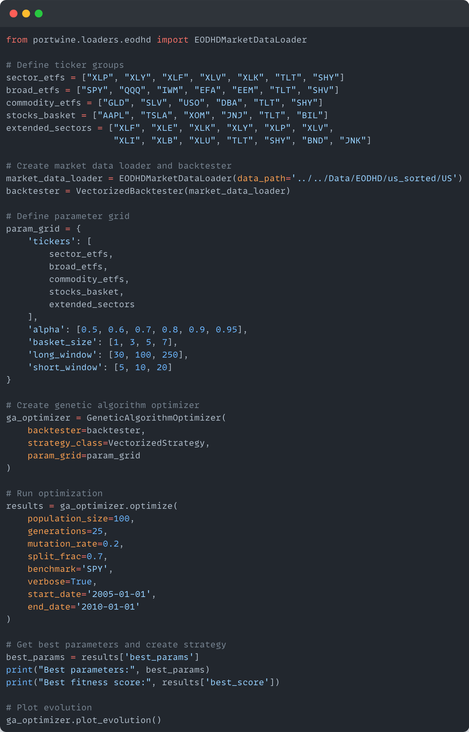
We have some parameters, different baskets, window lengths, etc. And then we put it into our optimizer (in this case a genetic algorithm optimizer) and get back our optimal parameters.

Best parameters: {'tickers': ['GLD', 'SLV', 'USO', 'DBA', 'TLT', 'SHY'], 'alpha': 0.95, 'basket_size': 1, 'long_window': 100, 'short_window': 20}

But, unfortunately, when we go to check the equity curve we get the following:

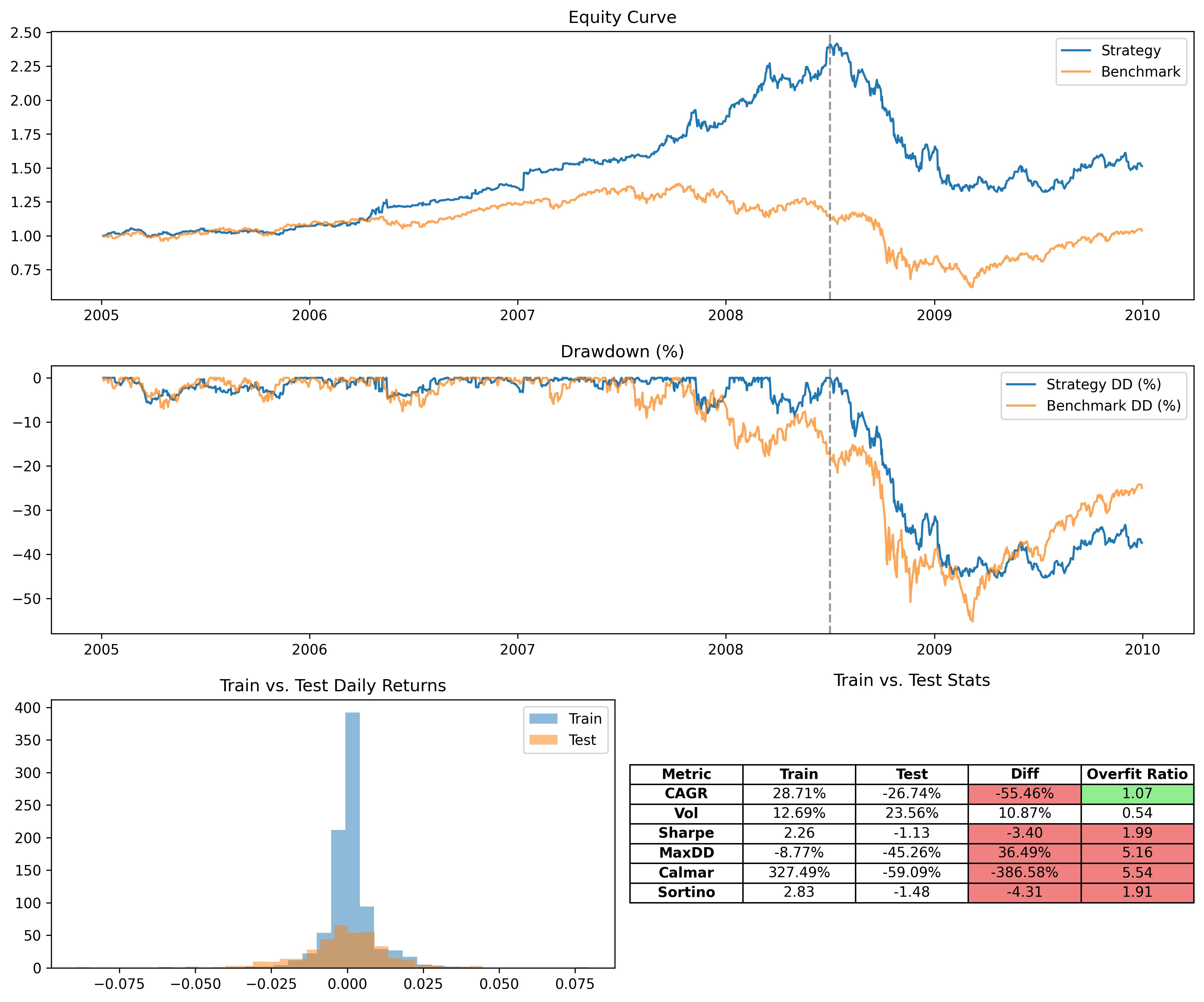
The strategy does great, right up until the 2008 Financial Crisis, and then it collapses. This is unsurprising as the data learned about a market condition that was never happened until 2008 (or at least with the data I gave it), so it was never able to learn what do to in such a situation (like most other people up unto that point).

Thus, I optimized a large amount of parameters to fit a very specific point in time that performs extremely well then, but collapses immediately after. We need to have a defense against things like these if we are going to deploy strategies into the wild.

It depends what you want to do. Does your strategy generalize itself or base itself off of general market factors that are constant? Or does your strategy need to ‘retrain’ it’s parameters every so often? Each one offers a different solution.

Let’s start with the first. Let’s assume that you have some sort of model that uses some sort of market factor like mean-reversion, momentum, etc. that is pretty consistent regardless of the regime. So, in this case, the model is probably overfitting simply because you do not have enough data points in the training sample. Let’s rerun the optimizer with a wider start and end date and see what happens.

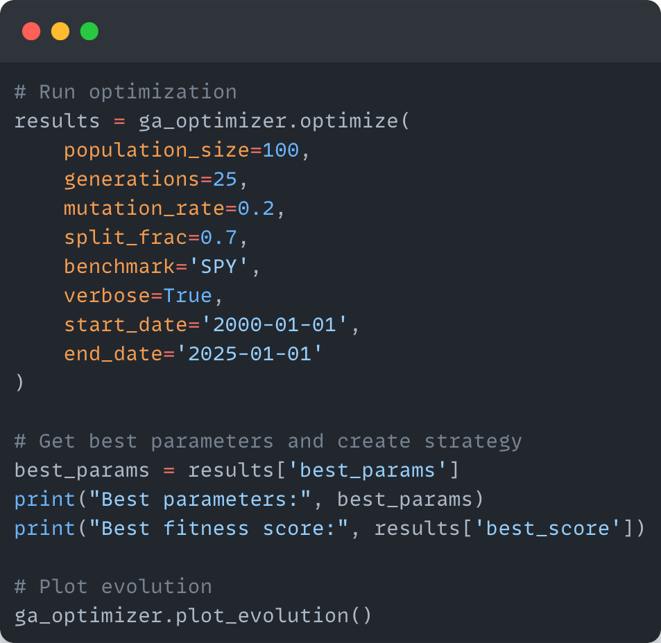
Best parameters: {'tickers': ['AAPL', 'TSLA', 'XOM', 'JNJ', 'TLT', 'BIL'], 'alpha': 0.7, 'basket_size': 5, 'long_window': 100, 'short_window': 10}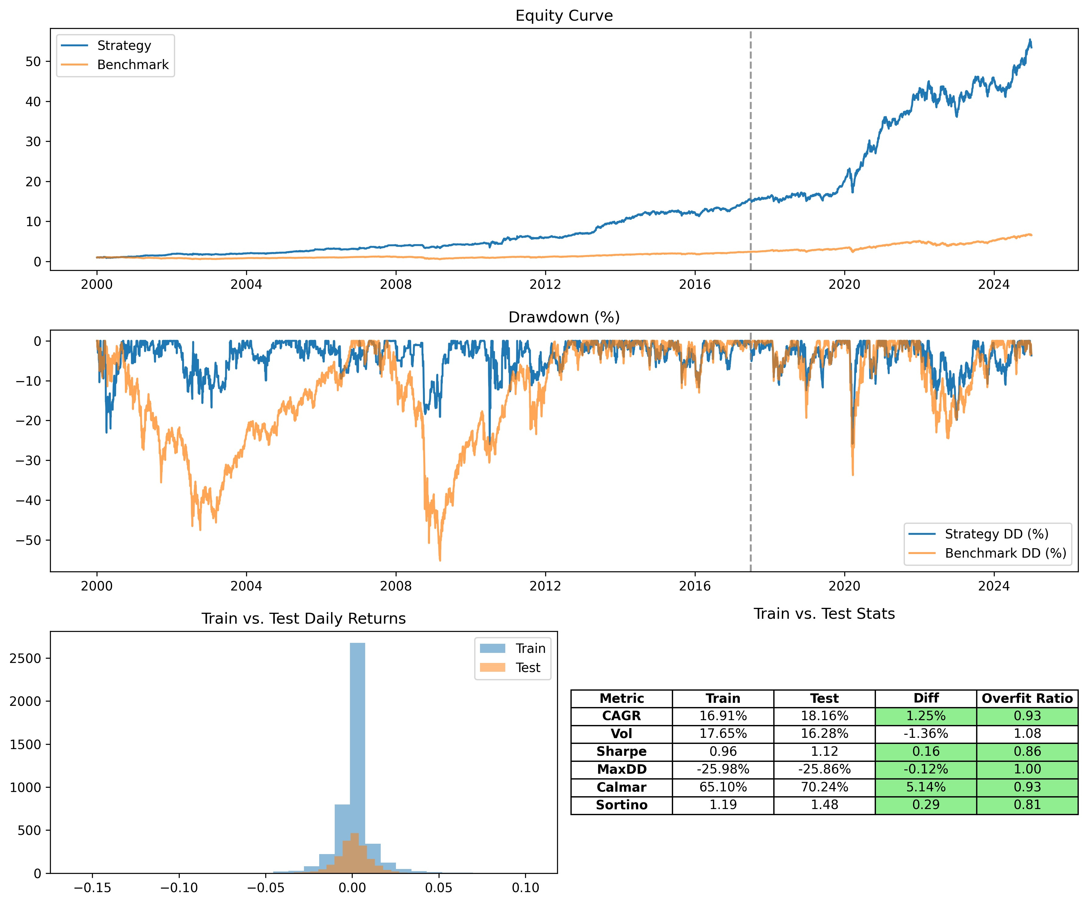

Easy. Now our system performs well through the 2008 Financial Crisis and shows low overfit into the future, including the 2020 COVID Crash.

Walk-forward Optimization

But what about systems where the optimal parameters change over time? Well, that’s where Walk-forward Optimization comes into play.

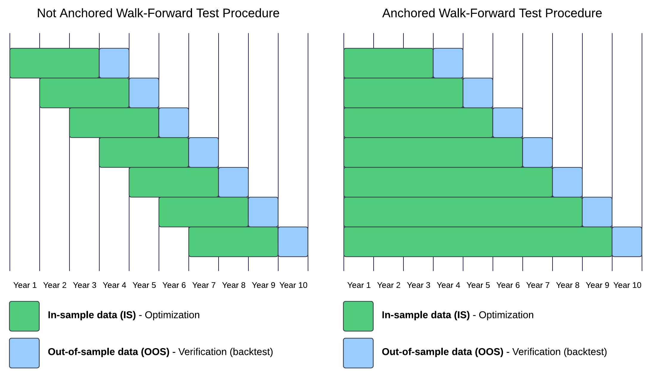
Walk-forward optimization takes a sliding or anchored window of data to train the model, then tests it on a small out-of-sample set to prove efficacy before continuing forward. This test can be used to make sure your re-optimization cycle does not create overfit solutions.

It also helps prevent look-back, as it simulates how things would work in the real world, generally. Generally, you would take a model, train it on all the data you have at that time, then let it run for a certain period of time before retraining it with the new market data to improve it.

Thus, by modeling this behavior before we go live, we can see the evolution of our system over time as it adapts to new data. Let’s give it a try.

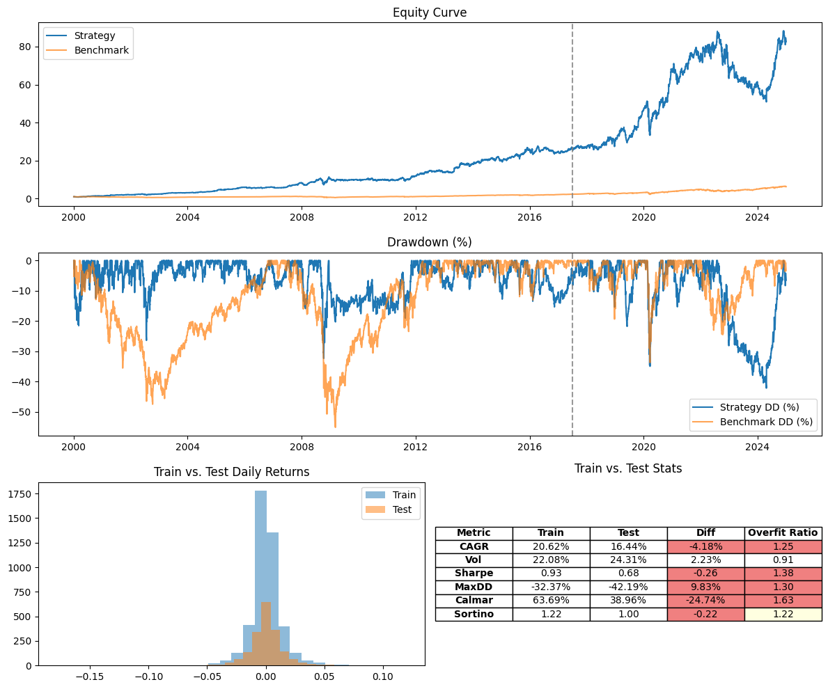
Here is another strategy that I have that uses a simple technical indicator. When trained on 70% of my data from 2000 - 2025, it looks good if I don’t consider the split. However, when I do, I see that all the metrics are decaying.

My strategy might perform better if it retrains every so often using the current dynamics of the market. You can see that most of the deviation was at the end of the out-of-sample data. So maybe the model is only fresh for a certain period of time? Let’s run a walk-forward analysis and see…

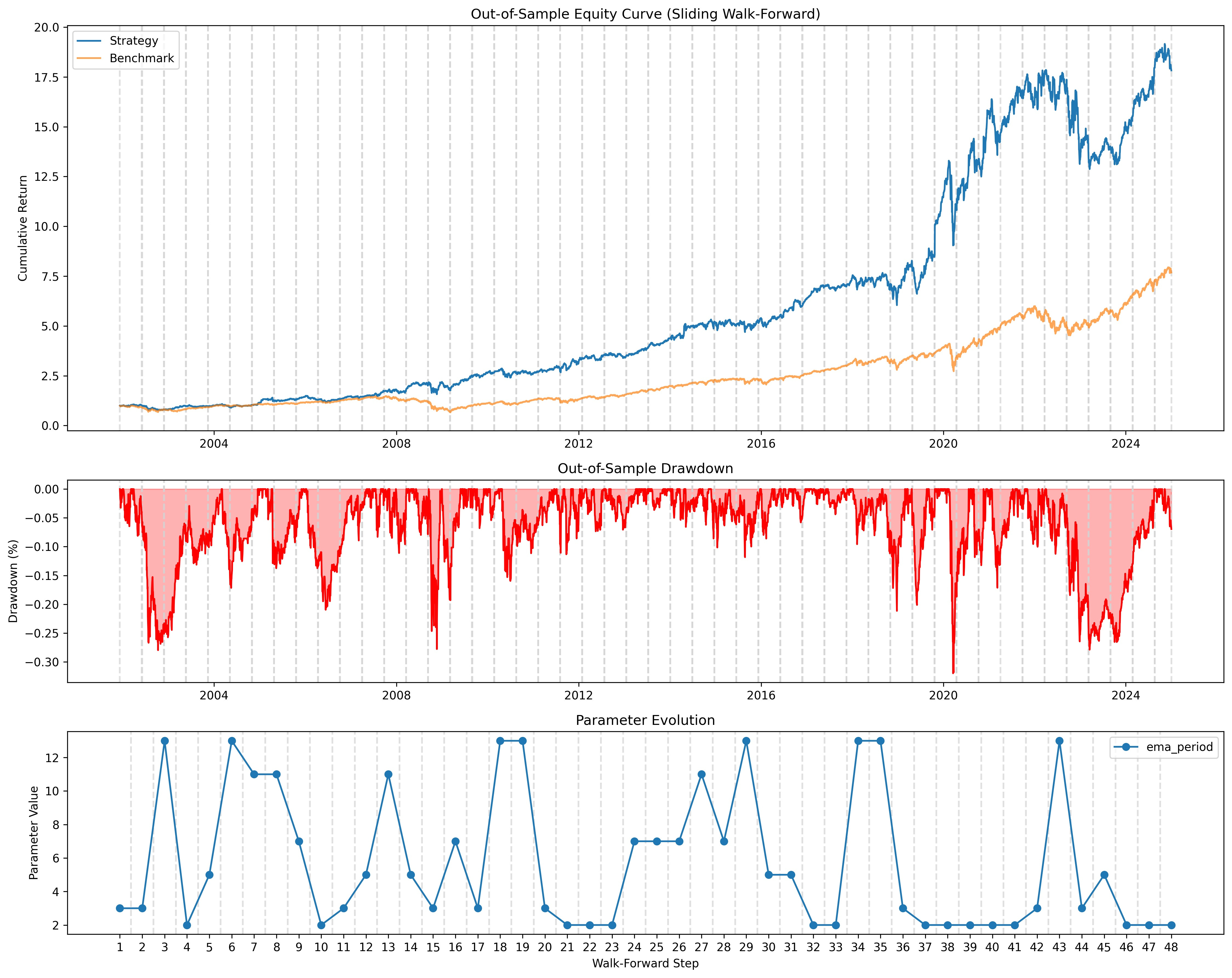
I set the walk-forward optimizer to non-anchored with a training set of 2 years and a test set of 6 months. You can see over time how the ema_period evolved in the lower chart. You also have to admit that the performance is not as good as the original overfit chart. But, keep in mind, the training set was overfit. If we analyze the data at the original split point (70% / 30%), we can compare the two and see how the walk-forward optimizer affected overfit.

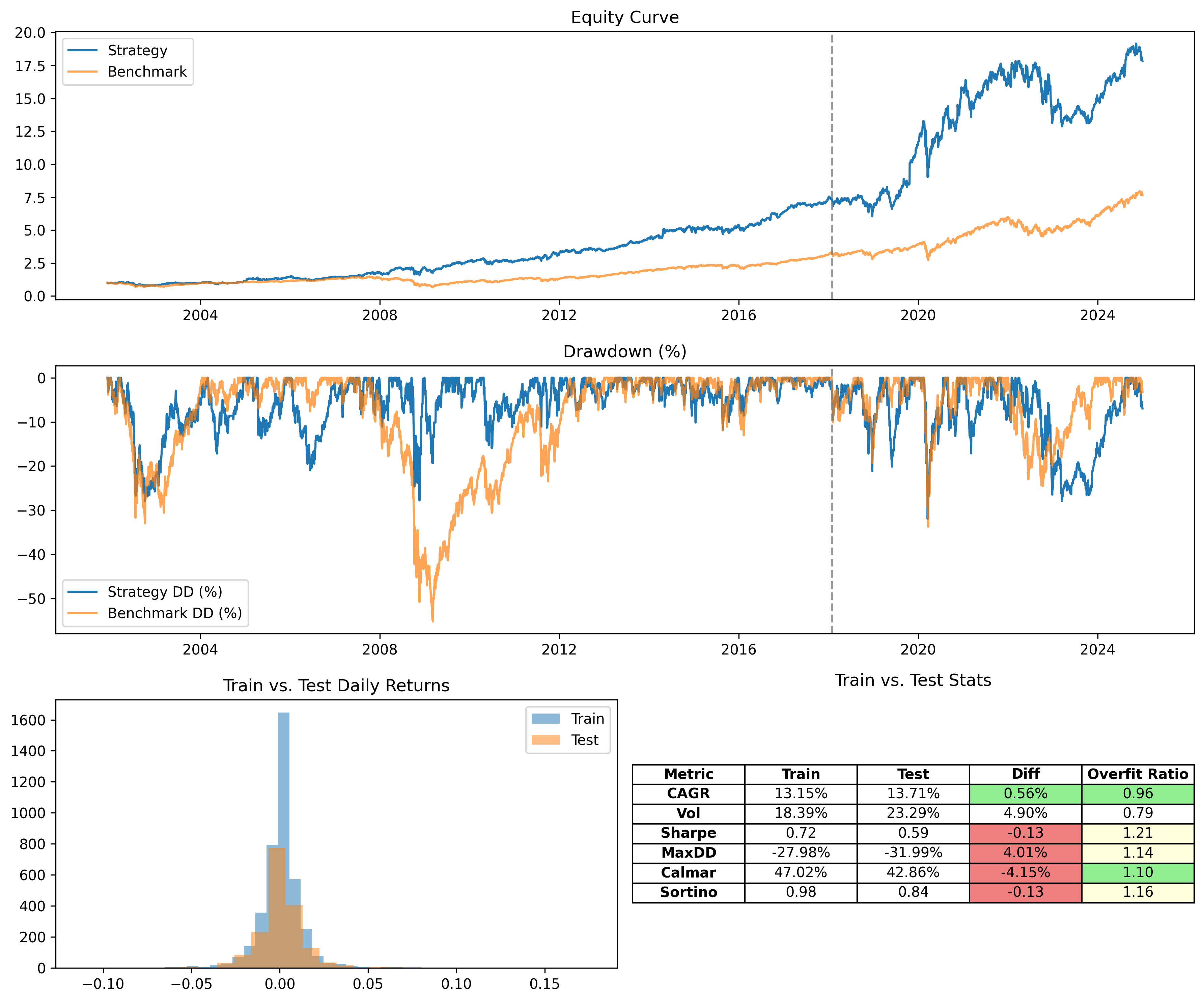
While the metrics are not as high as the run before (test CAGR is 13.71% instead of 16.44%), we have much higher stability. None of the parameters are overfitting. There are decreases in some of the metrics between the train and test sets of the walk-forward results, but within acceptable levels. This demonstrates the walk-forward optimizer’s ability to combat overfit.

From here, we can experiment with different train and test sizes, hyperparameters of our optimizer, etc. until we get the optimal curve that hits our target CAGR and other metrics while retaining high stability and most of all, avoiding overfit.

Because we know that the walk-forward optimizer handles overfit inherently, we can throw all of these hyperparameters at it and not worry what comes out. That is not the case with a simple train-test split.

Conclusion

In conclusion, overfitting is a monster that we are all afraid of. However, with the right tools, you can avoid the common pitfalls and failure points that many of us end up getting stuck in.

Look out for part 3 that goes into modeling and simulating certain market dynamics which can also bolster the confidence you have in your trading system or reinforce it even further.

If you want the code for the walk-forward optimizer and genetic algorithm optimizer, become a paid subscriber today. Your support help me continue my research and deliver you the most impactful information that you can use in your quantitative journey to profit.