Taming OLMAR’s 1222% Backtest into a Sustainable 106% CAGR

Mean reversion: the secret sauce to sustainable alpha.

Often as traders, we equate complexity with profitability. A model’s edge comes from it doing something that no other person on Earth has tried yet. But the data shows that simple rules based on real market factors still outperform most models. Those that continue seeking complexity are headed towards a dead end.

---

Today I’m focusing on the Online Moving Average Reversion (OLMAR) system by Bin Li and Steven Hoi, an online portfolio selection system that drastically outperforms the market in most examples. It’s a brilliant piece of math from two authors that are top of their class in online portfolio selection algorithms.

But here’s the kicker:

This strategy is not based on some wild, unknown alpha using crazy state of the art machine learning techniques. It’s based on simple mean reversion and price data only. And it gets 106% annually.

First Step - Understanding Mean Reversion

Before getting into the mathematics, let’s learn about mean reversion, which underpins OLMAR.

Mean reversion is one of the major market factors that describes an asset price’s tendency to “snap back” toward its historical average after drifting too far up or down. Think of it as a rubber band: stretch it too far and it will pull you back.

You probably have heard things like the ‘Dead Cat Bounce’ which states that when there is a massive crash, there is generally a ‘bounce’ back period. This is a type of mean reversion

You also have heard about ‘buying the dip’ because the market ‘always recovers’ over the long term. This is especially true for major market indexes like the SP500. You probably recently seen a ton of posts about this regarding the Trump tariffs as a way to calm down the markets.

Specifically defined, mean reversion is made up of two parts:

• Mean - a long-run average level (e.g. the 200-day moving average).

• Reversion - the force that drives price back toward that mean.

(Crazy, I know.)

But what makes mean reversion different than a technical indicator is that it is empirically proven to have significance. This behavior is time and time again proven in research to exist. That is why it is so important to understand it.

Why Does it Happen?

There are many real economic and behavioral factors that explain why mean reversion occurs and why it will continue to occur. Consider the following market participants and their motivations:

1. Value Traders

   1. Institutional investors often target fundamental valuation metrics (P/E, dividend yields, book-to-market).

   2. When prices stray too far from fair value, value‐oriented investors either buy them back up to the fair value, or sell them back down to the fair value.

   3. Fair value can be some internal model that they have calculated on a per asset basis

2. Reactionary Traders

   1. News, rumors, and asymmetric information can drive excessive buying or selling.

   2. Once reality sets in, the market corrects itself—traders “buy the dip” or “sell the rip.”

   3. Often the case for market crashes (recent tariff scare) or spikes (GME melt-up)

3. Risk-Considerate Traders

   1. Many funds maintain target exposures (e.g. “50% equities, 50% bonds”).

   2. If equity markets spike, rebalancing forces sell equities back toward targets; if equities crash, rebalancing buys the dip.

4. Market Makers

   1. Market-makers and dealers try to keep inventory neutral.

   2. Large one-sided order flows force them to lean against the move, supplying or demanding liquidity that nudges price back toward average.

   3. That means that if a single position starts to take up most of their gains (because it is rapidly increasing in price), they will unwind some of their inventory to keep things neutral.

How Mean Reversion Prints - an SPY Example

Let’s take a real world example: let’s buy and hold SPY for 1 day whenever the price dips 2% or move below the 20-day moving average.

Thus:

1. Enter when SPY close is less than 98% * 20-day moving average of SPY

2. Exit 1 day later

Here’s what that looks like in practice:

Although we are only in the market a small percentage of the time, we make considerable returns over the last 25 years.

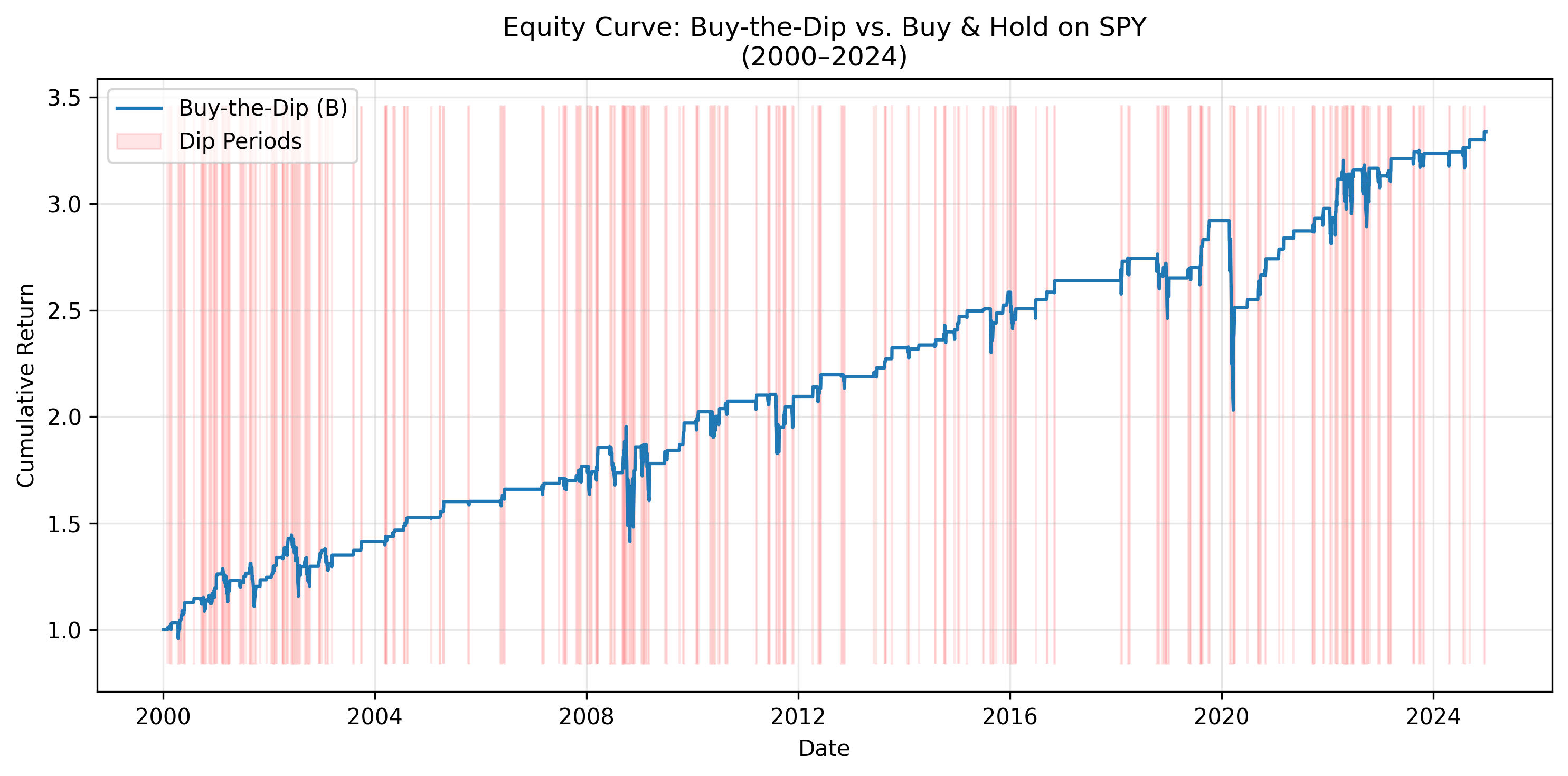
Some markets do better than others with this simple strategy. The SPY, because it is the general market index, probably performs the most consistently because this strategy captures the general ‘buy the market when it goes down because the market always recovers’ trope that many traders have.

For example, GLD shows some alpha with this strategy:

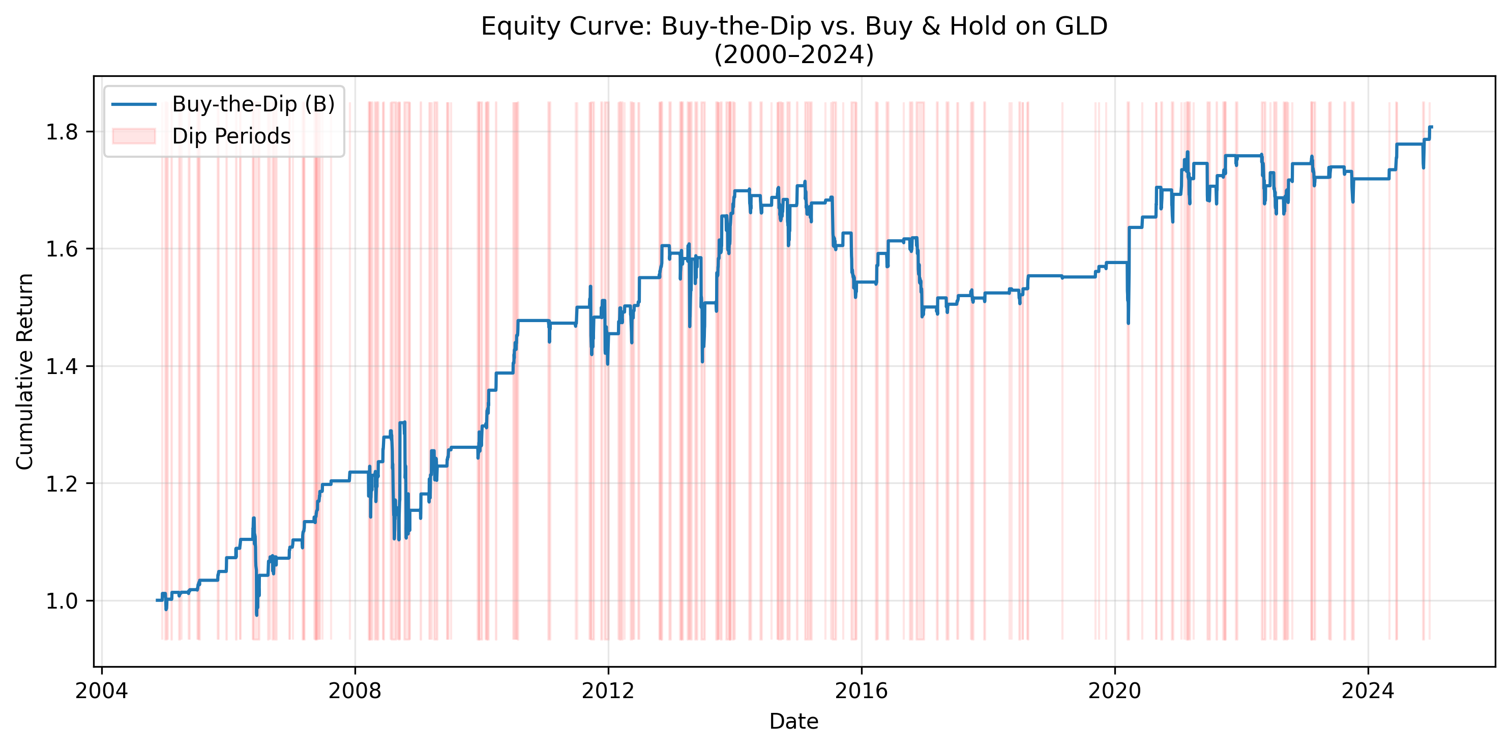
But it is not the same consistency as SPY (perhaps due to GLD having more pronounced upward and downward trends over longer periods of time).

Introducing Online Moving Average Reversion (OLMAR)

And so, now we know that mean reversion is a major factor in the market that can lead to profitability and we have demonstrated it working on the SPY. But can we create a more sophisticated system that exploits this market factor?

The answer, of course, is yes. And the answer to that is the OLMAR system.

Bin Li and Steven Hoi out of Nanyang Technological University in Singapore devised this online portfolio selection system that takes exactly this factor into account, exploiting assets’ tendencies to revert back to their moving averages (hence the name). They outlined their system in a paper titled On-Line Portfolio Selection with Moving Average Reversion back in 2012 and I encourage you all to check it out. Li and Hoi’s work in online portfolio selection in general is top tier.

The system is simple.

1. Get the current prices for assets in your basket for the current trading day.

2. Compute the updated moving average for each (window size is a variable).

   1. For assets trading above their moving average, we expect them to come down.

   2. For assets trading below their moving average, we expect them to come up.

3. Calculate the ‘expected returns’ for each asset.

   1. This is the percentage difference between the assets’ current prices and their moving averages.

4. Get the portfolio’s ‘expected returns’

   1. Apply those returns to the current portfolio’s weights (returns × weights).

5. Buy low, sell high

   1. Adjust our weights to increase exposure to underperforming assets and decrease to overperforming ones.

6. Repeat for tomorrow (go to step 1)

Over time, the portfolio evolves and adapts based on the market conditions.

Theoretical Potential - 1222% CAGR

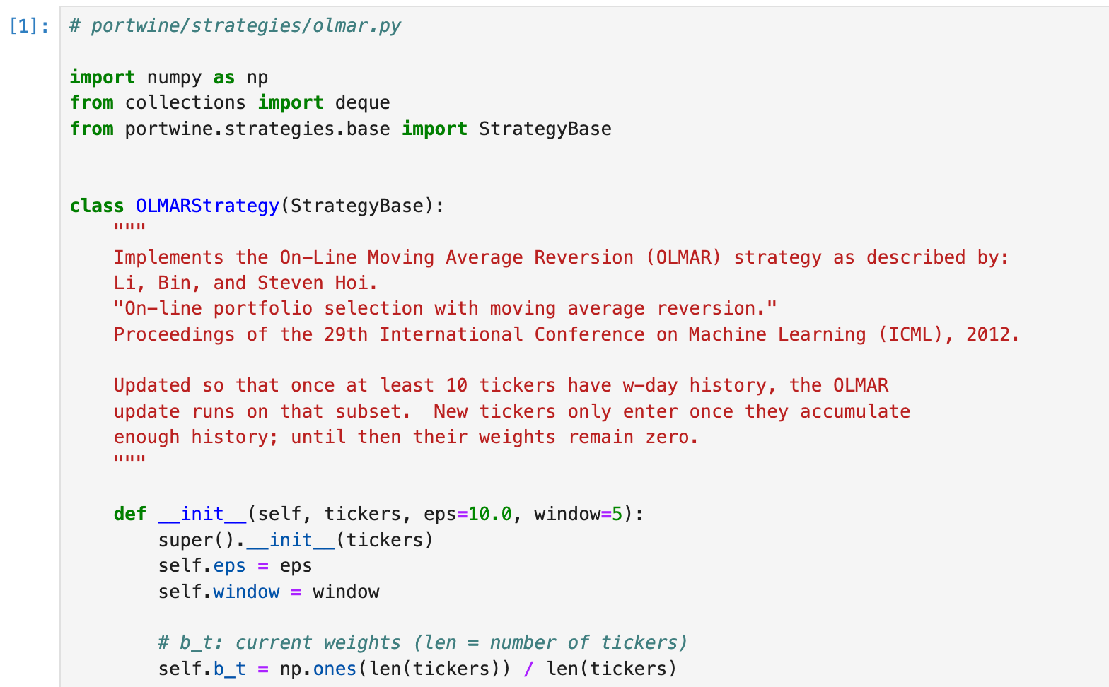
I coded this strategy, faithful to the paper, in my portwine open-source backtesting library (available here) and ran it on the SP600 Small Cap constituents. The paper uses the NYSE, Dow Jones, and TSE, however I wanted to try something different so see if it generalized to other markets.

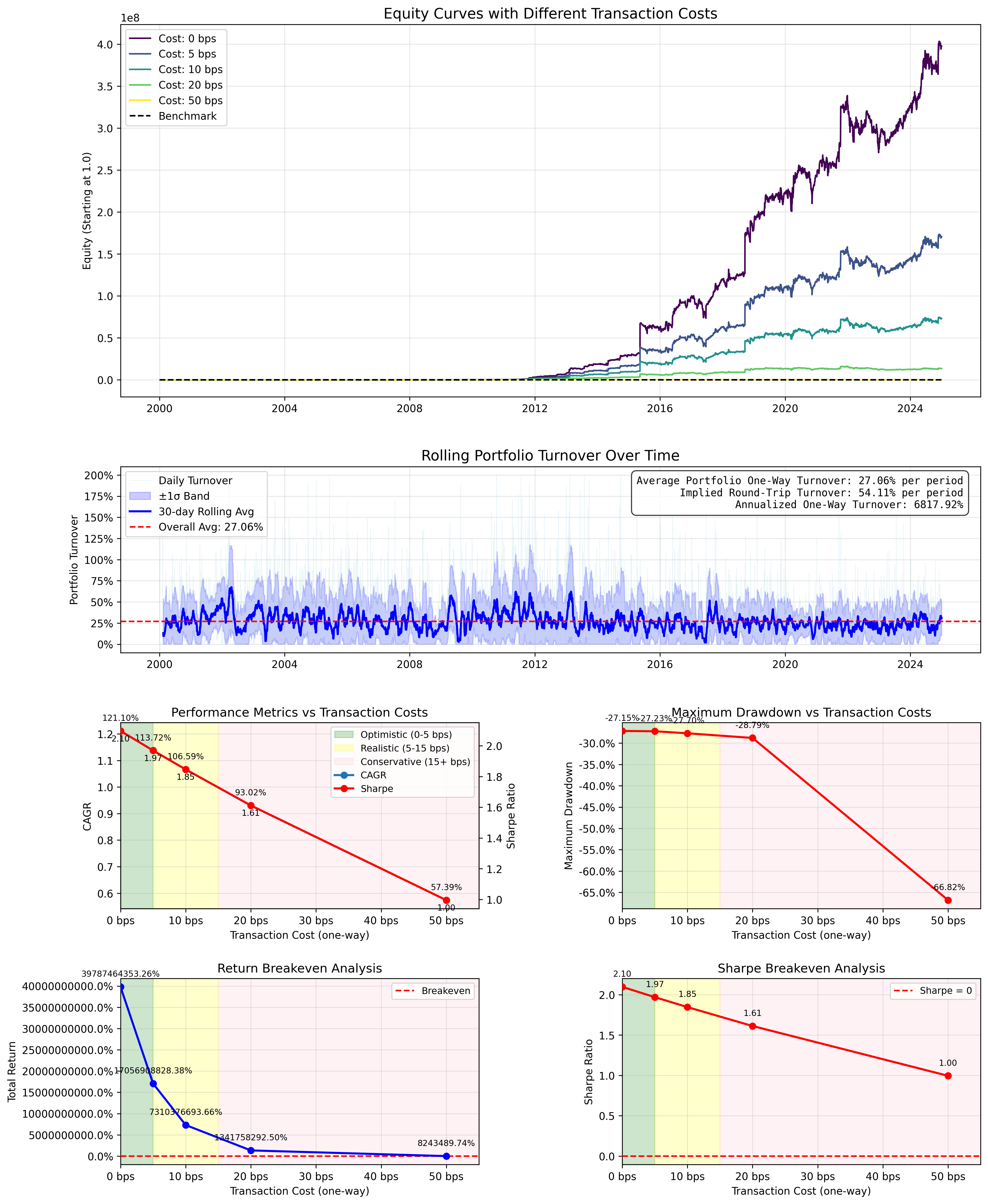
So, I set my moving average window to 25 days, and fed it the SP600 components. This is what came out:

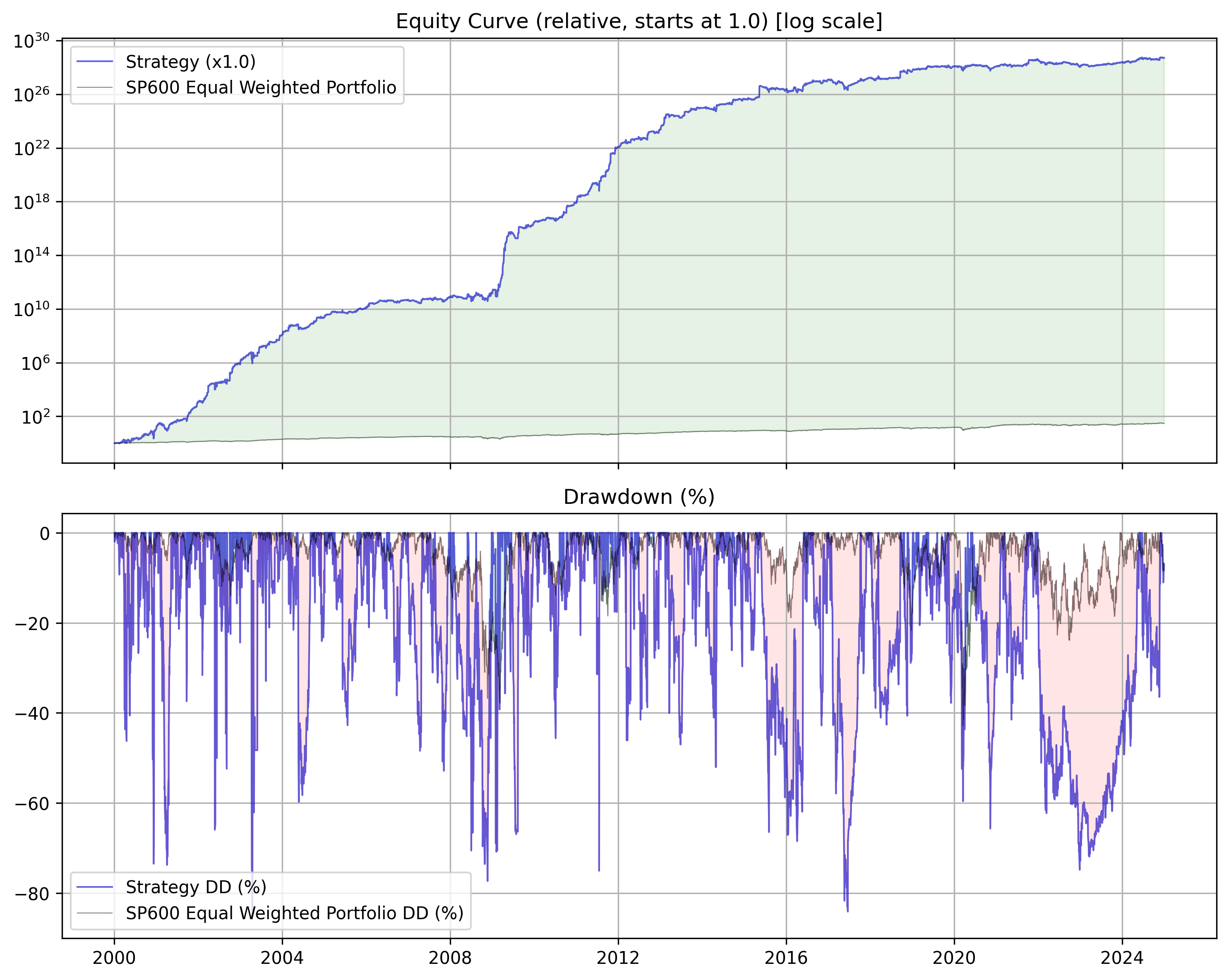
Yes, you’re seeing that correctly. That is 10 to the 30th power, or 10 with 30 zeros after it in total returns. So I guess you could say this strategy works extremely well. However, the drawdowns are extremely painful regularly passing -75% for prolonged periods of time. And, transaction fees take out their fair share out of the performance.

The labels are totally messed up because I wrote this analyzer without ever expecting to encounter a strategy like this. But, here we are.

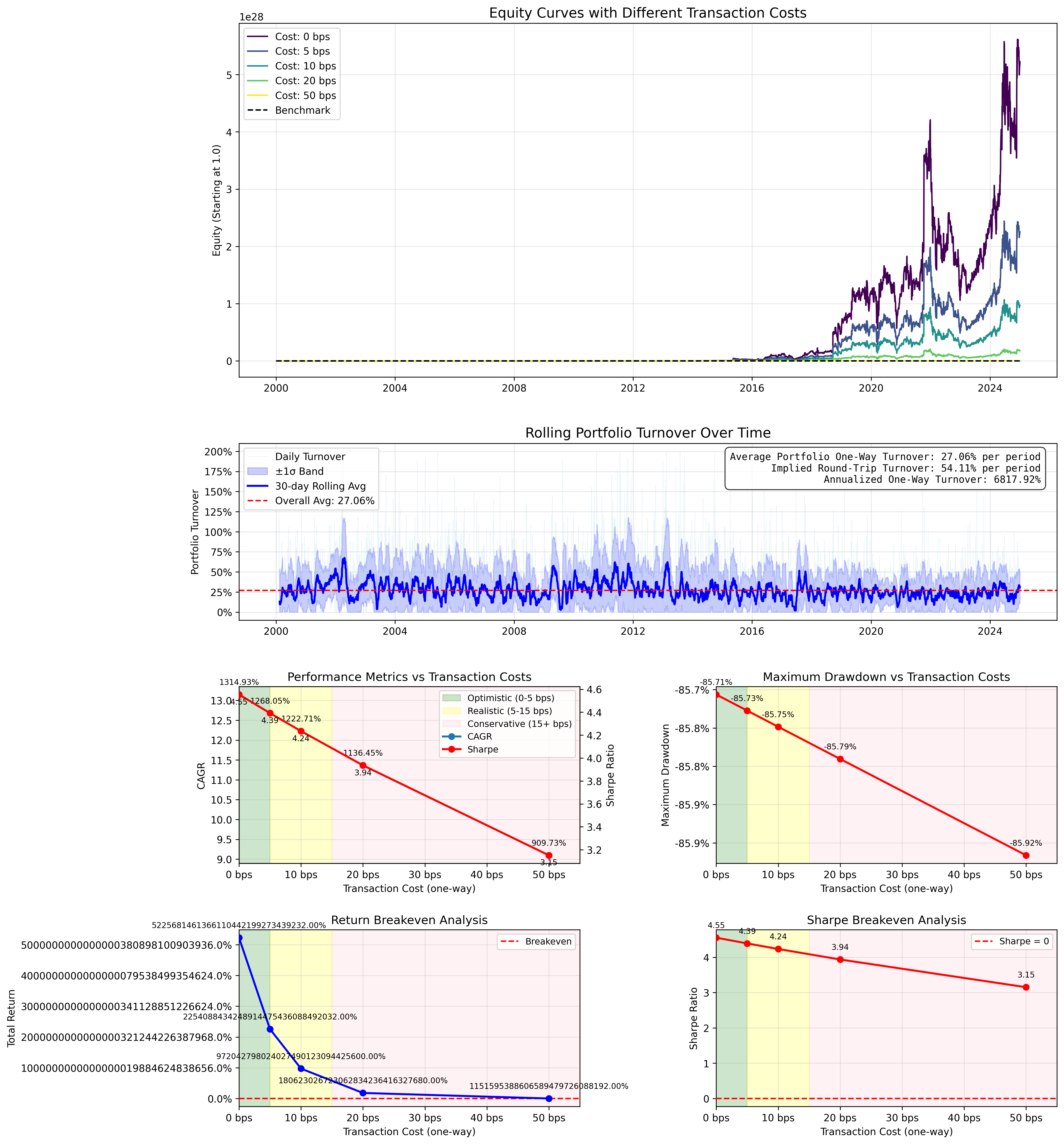
We have an annual turn over of over 68x, which means that we are flipping the entire value of portfolio every 3.7 days (252 trading days / 68 flips). This requires quite a lot of transactions, and thus fees.

But, because the performance of this strategy is pretty ridiculous, even 50 bps fees, which rarely every occur, still produce a CAGR of 909% (ignore the drawdown of -85% however).

These numbers are a bit nauseating. It would be great if we could dial down the insanity at the expense of potential upside. The volatility of this thing is too extreme.

I decided to decrease the leverage in an attempt at reducing our drawdown and risk. I decided that if we only traded 20% (0.2x) of our capital at a time, and kept the rest in a risk free asset (assume cash for now), then we could capture a lot of upside, theoretically 240% CAGR, with reduced drawdown, theoretically -17% drawdown.

This is the best of both worlds- stomach-able drawdowns with still well above average returns. Thus, I wrote a snippet to modify the leverage of our results from the strategy:

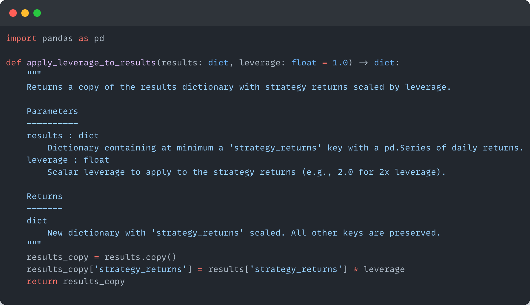
Which assumes we only ever allocate a total of 20% of our capital into this strategy. The results are much better.

Reaching Stability - 0.2x Leverage

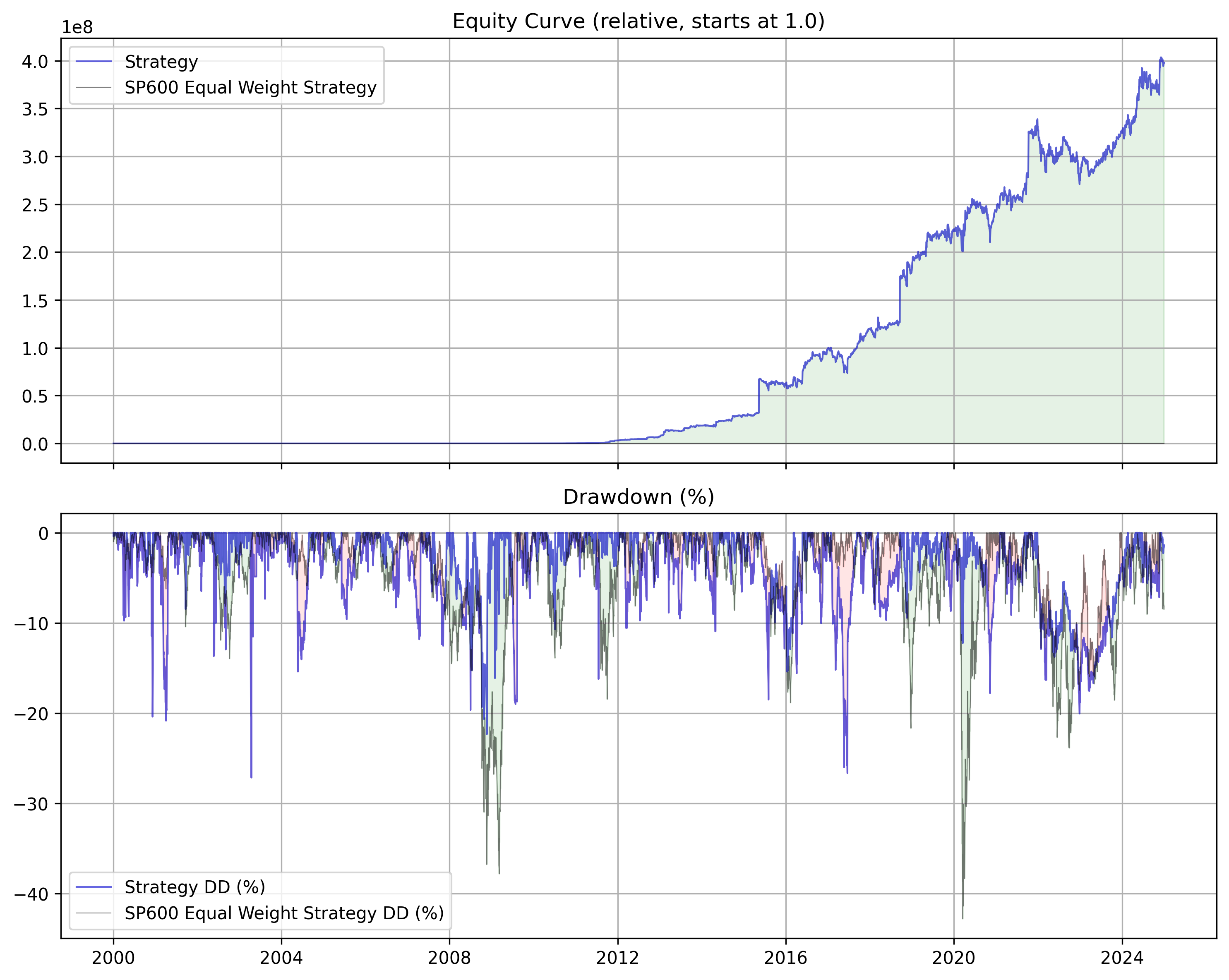
As predicted, our drawdown is much lower, and even lower than the equal weighted benchmark. But we still have tremendous upside.

And while it’s not the theoretical numbers that I spitballed, we are still getting 106% CAGR at 10 bps transaction fees (a reasonable assumption) with -27% maximum drawdown which is well below the benchmark.

This showcases that OLMAR is still a great online portfolio selection algorithm that is simple, versatile, and highly profitable in general markets over 10 years after being published.

Next Steps & Getting the Code

1. Try It Yourself

   • Grab the full Jupyter notebook, including live data loaders, visualization cells, and the production-ready OLMARStrategy implementation.

   • Tweak your own baskets—whether it’s tech, dividends, or global commodities—and see how the system balances them in real time.

2. Join the Inner Circle

   • Paid subscribers get immediate access to the private Google Drive, where you’ll find:

     • The complete OLMARStrategy module for Portwine.

     • Visualizations and analyzers not included for free subscribers that you can use in your own systems.

     • Access to the archives of all strategy code from all previous posts.

Thanks again to all my subscribers, paid or free, and happy researching!