I Used a Thermostat’s Logic to Control My Portfolio—And Achieved 24% CAGR

Turning Temperature Control into Market-Beating Performance

An appropriate system in time for the heat of the summer.

As traders, we scour the internet, books, and articles for industry specific information to create our new fancy algorithms. The Black-Scholes model, Markowitz Mean-Variance portfolio optimization, the Capital Asset Pricing Model (CAPM)… These are all systems designed for investment purposes solely.

Enough of this math nonsense. We need something more tangible.

But what if solutions from a completely different domain, ones that seem completely detached and even too simplistic to make an impact on any investment decision, turn out to outperform many of these established models?

Now, this makes much more sense to me.

I discovered that the same system to maintain the temperature of your house is adaptable to markets, and not just by a small edge either. The data shows 24% CAGR on SP500 components, beating an equal weight strategy by 2x.

We’re often quick to dismiss out-of-the-box thinking or get stuck in the trap of ‘industry knowledge.’ But doing so ‘boxes’ us into rigid thinking patterns that every other trader uses, and thus provide no novelty and stale alphas that have been priced into the market for decades.

Here’s the thing:

Being open to concepts and ideas that are not part of the norm is often seen with ridicule and rejection. But, they are often the holy grail of alpha. Creativity, persistence, and ingenuity is what separates the good from the great.

And here’s how I did it.

Thinking in Thermostats

Behind every thermostat is a simple system. If the air is too hot, it turns on the air conditioning. If it is too cold, it turns on the heat. Of course, the A/C and heat take time to turn on and off. And so, often times the thermostat might ‘overshoot’ or ‘undershoot’ that comfy target of 21°C (72°F).

Comparison of different controllers (P, PI, and PID controllers) adjusting a thermostat.

The class of systems that govern this behavior are known as Proportional-Integral-Derivative Controllers. These controllers take into account:

1. The current error of the system (Proportional)

   1. What temperature it is right now versus what temperature we want.

2. The accumulated error of the system over time (Integral)

   1. How long as the temperature been off target.

3. The rate of change of that error (Derivative)

   1. Are the settings of the system making things better or worse?

These factors are added together to create a total error which influences what the system should do next.

This feedback tells the controller whether to increase or decrease the heat, by how much, and how quickly.

Visualizing with Boats

The same problem exists in navigation. A boat’s rudders need to maintain a certain heading. But, ocean currents and winds push the boat off course and the rudders need to compensate.

To illustrate how PID controllers work, I made a visual example. Our boat’s target heading is set at 45 degrees and I added simulated currents to attempt to push the boat off target. Here’s the path of our ship.

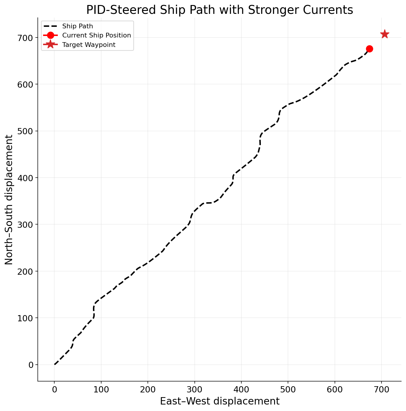
You can clearly tell how there are periods where the boat is wavering from it’s target waypoint (45 degrees forward). But, over time, it nudges back over to the target and continues it’s path.

You can see the PID controller working under the hood here:

Let’s go through each graph together.

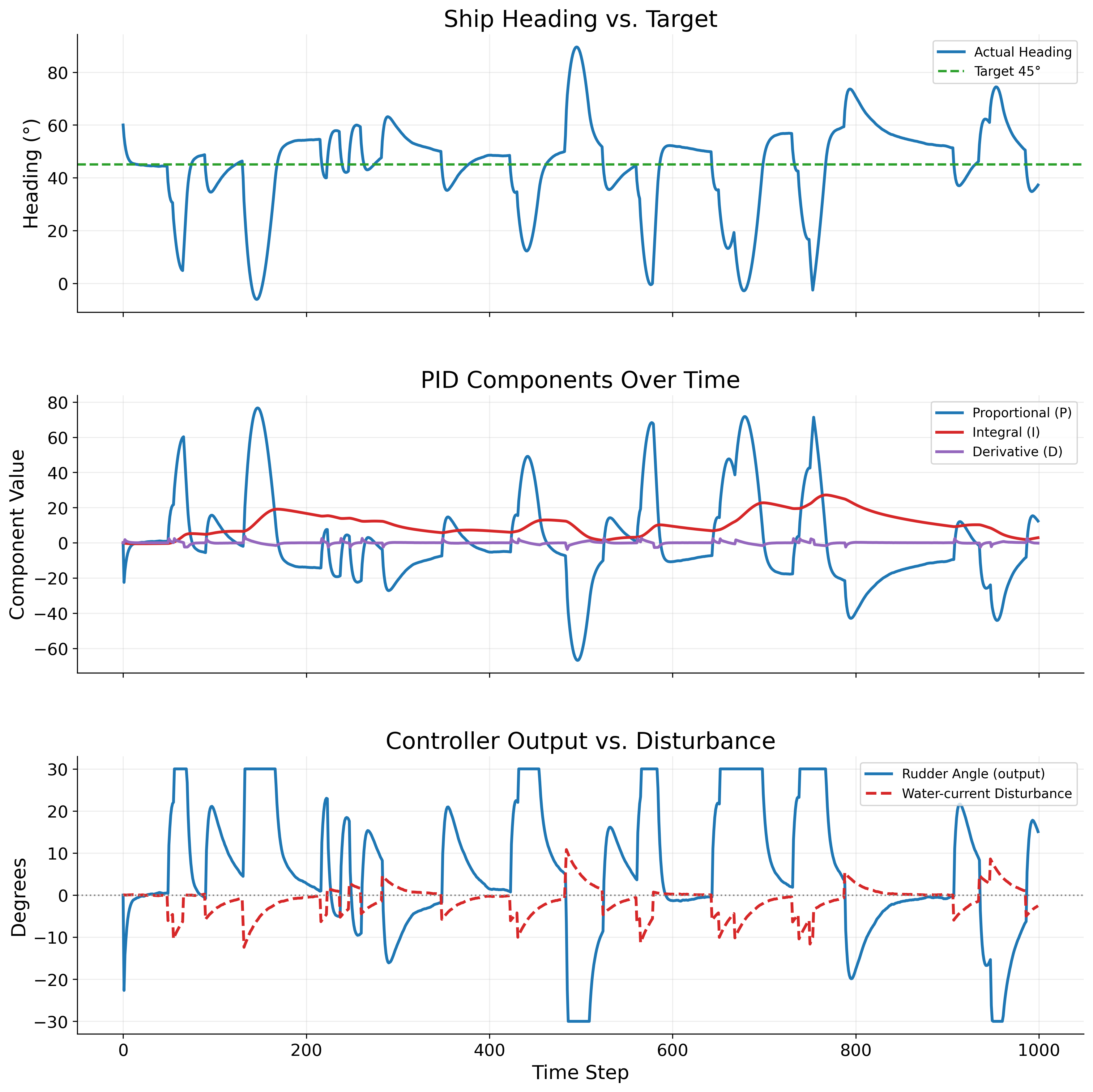
Ship Heading vs. Target

This plots the direction that the boat is heading over time. The sudden dips and spikes are the programmed currents knocking the boat off course. But each time, the PID controller adjusts the rudders to compensate such that the heading is realigned to the target, denoted by the green horizontal line.

PID Components Over Time

This plots the ‘under the hood’ components of the controller. You can see the proportional error which spikes immediately in the opposite direction of the heading. This is because if the boat is pushed to the right, we need to knock it to the left. Thus, the action is the opposite of the error that we need to take.

The integral error is the accumulated error over time. Or, how much are we off from our target in total? This tells the controller how to react after we immediately react to the sudden currents. After we adapt to that sudden change, are we still off course? How to we slowly turn the ship back on course over time?

The derivative error is the change in our error. You can see how it spikes with the proportional error, but very quickly levels back off to around zero. This is helpful for the system to react extremely quickly, or to understand in what way the error is being applied to the system (quickly or slowly).

Controller Outputs vs. Disturbance

This plots the actual ‘shocks’ or current disturbances and the end action that the rudder takes to adjust for these shocks. The rudder’s actions are clipped at 30 degrees either way, as is the case with real world rudders and prevents over compensation which would spin the boat totally out of control.

You can clearly see how the rudder quickly adapts to the shocks, and then slowly readjusts to 0 as it gets closer to the target heading, just like how a real boat’s navigation system would work.

Applying to the Markets

But sure, boats and theromstats are cool. But what does this have to do with markets? They are hardly the same thing. There is no fixed ‘target’ of where we are heading. Markets are chaotic and constantly dealing with shocks and unexpected behavior. The problems are completely different.

A classic visualization of chaos theory and how simple rules can lead to high complexity.

That might be so. But, the PID controller is actually a great adaptive system for the markets.

I made a simulation where the target of my controller was a Sortino ratio that was high enough to promote the controller to accumulate wealth without the error being absolutely insane where the controller doesn’t know what to do.

I also constructed three assets: Asset A, Asset B, and Cash. The system could allocate in any of these assets over time. The system only knows the three components (P, I and D) of how off it is from the target.

To illustrate this better, I added regimes to Assets A and Assets B and alternated between them:

1. Asset A outperforming Asset B

2. Asset A underperforming Asset B

3. Both Asset A and Asset B underperforming cash

This gives the controller different market conditions in which is has to adjust its weights to maximize wealth. Here’s what happened:

Each vertical line marks the change of regimes.

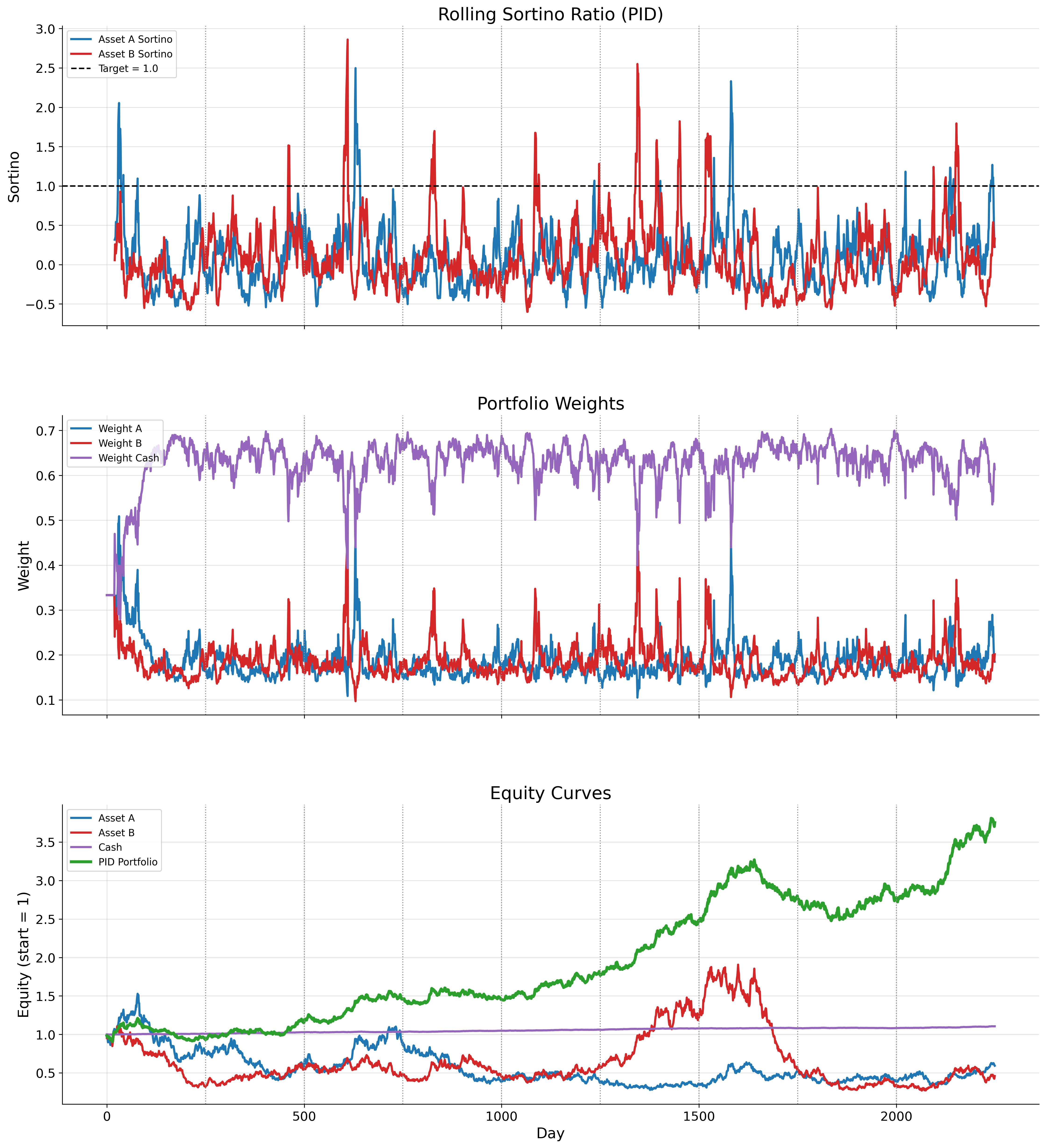
You can see the 20-day rolling Sortino ratio for each asset in the top chart which illustrates where the controller should be headed. And, unsurprisingly, the portfolio weights shift from Asset A to Asset B when the Sortino ratio of each asset adjusts.

You can see in the final plot how much better the PID controller performs that any of the assets, as it is tactically adjusting its weights based on how each asset is performing.

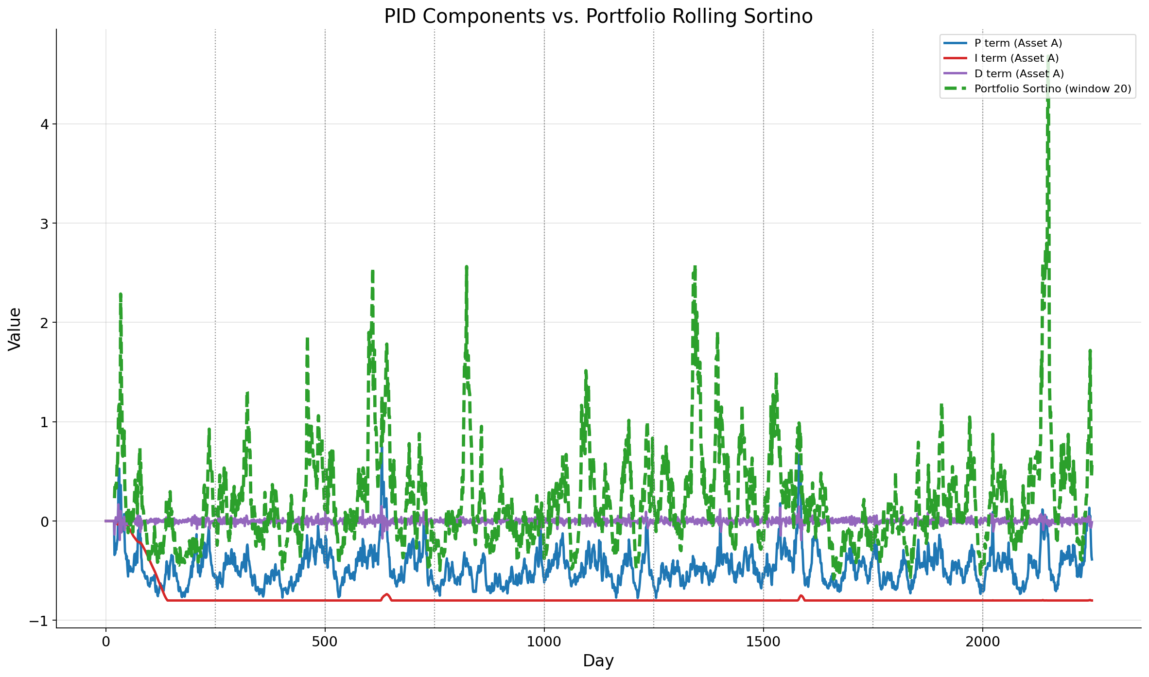
Above is a chart of the PID components and the rolling Sortino of the PID strategy itself. You can see that the proportional error adjusts often as the value of the portfolio changes over time. However, because the portfolio is often above the target Sortino ratio of 1, the integral error is constantly negative. This is good, as it means that the system, over the long term, is performing well. The derivative error is a bit harder to see, but you can see how it is quickly adjusting to the small daily movements of the portfolio.

Achieving 24% Returns on a Weekly Strategy

And so, I moved onto developing an actual strategy. This system was actually developed with the help of my automated research process, and so it’s great to see that such a powerful concept was able to come out from it.

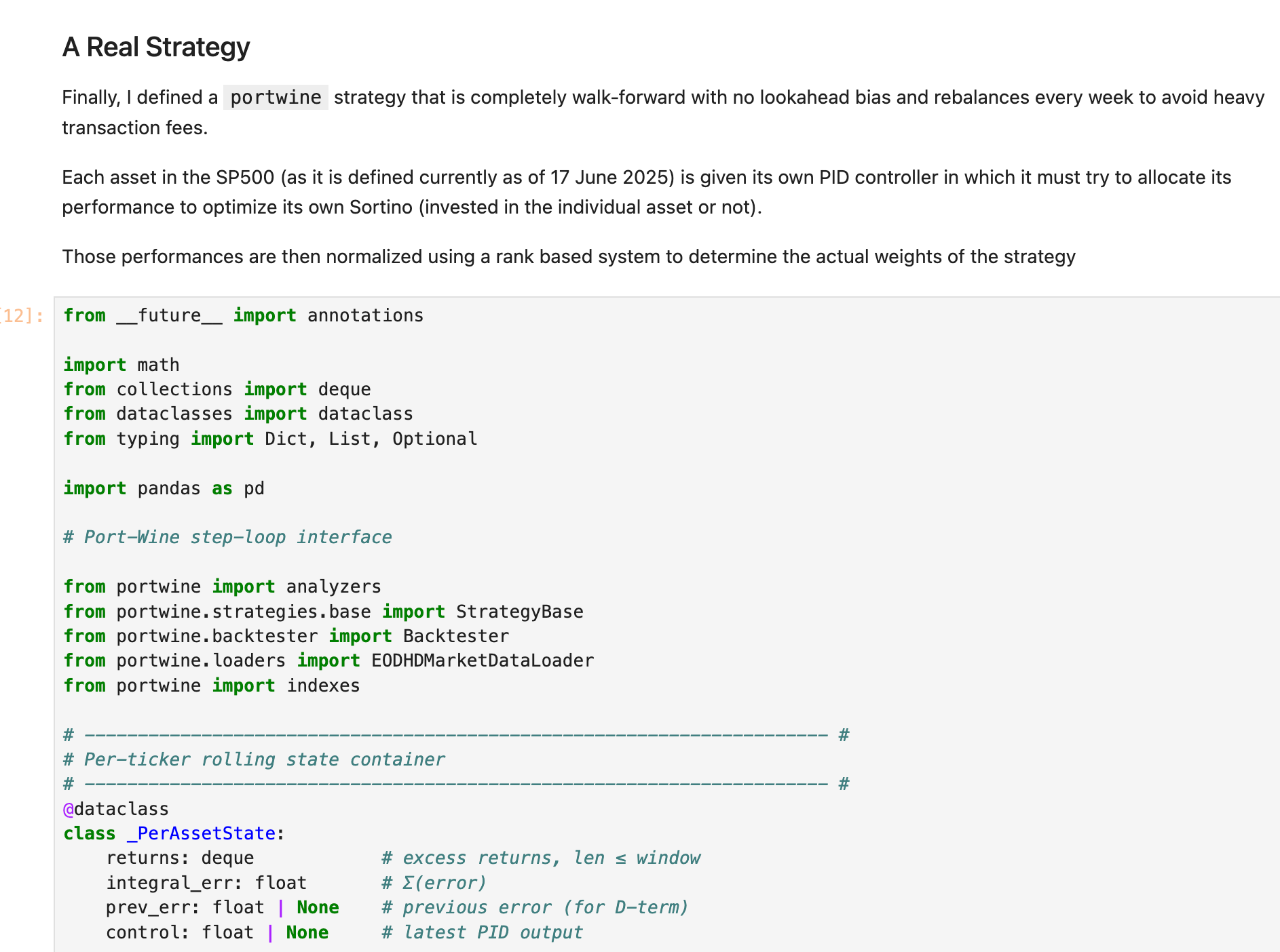
That being said, I incorporated the concepts here into a single system that trades all of the SP500 components (as of today) on a weekly basis.

The target metric is a Sortino ratio, just like the version above. Except, instead of the controller adapting at every time step, it only does every 7 time steps to avoid excess turnover and keep transaction costs down.

Furthermore, every asset has it’s own controller assigned to it such that the strategy is an accumulation of all the controllers at once. This allows for a per asset granularity of control that would be very hard to achieve otherwise.

I used exponential ranking to then take the performance of each PID controller and map it to portfolio weights.

Results

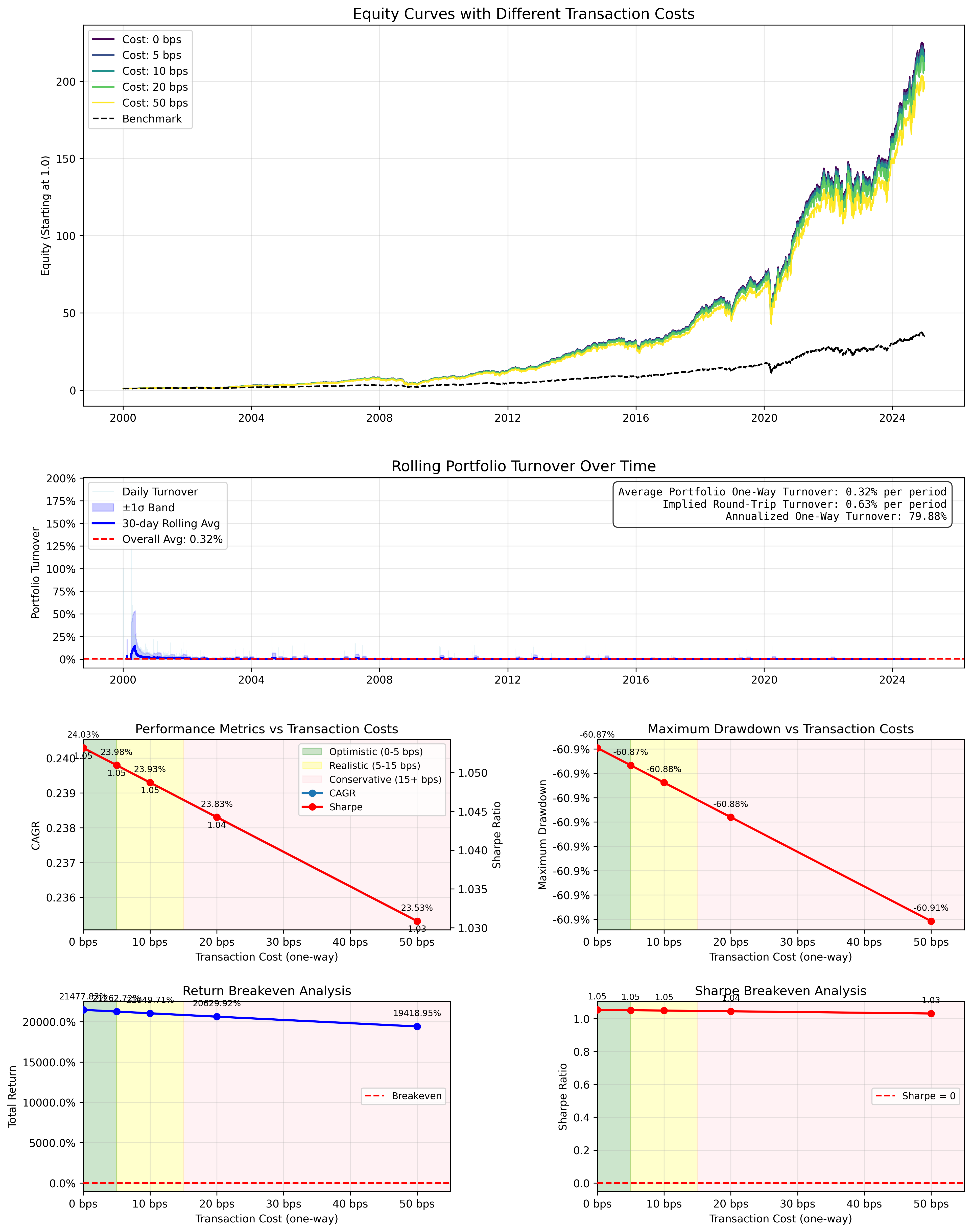
The system performs extremely well, while being a low frequency strategy with very low turnover. This illustrates the effectiveness of the PID controller.

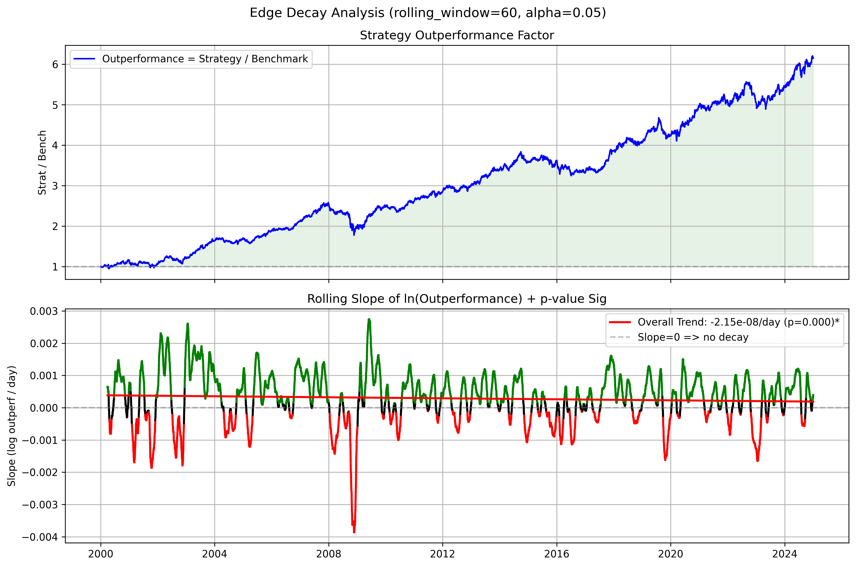
And, when comparing the edge of this system against an equally-weighted one of the current SP500 components, we see a steady edge:

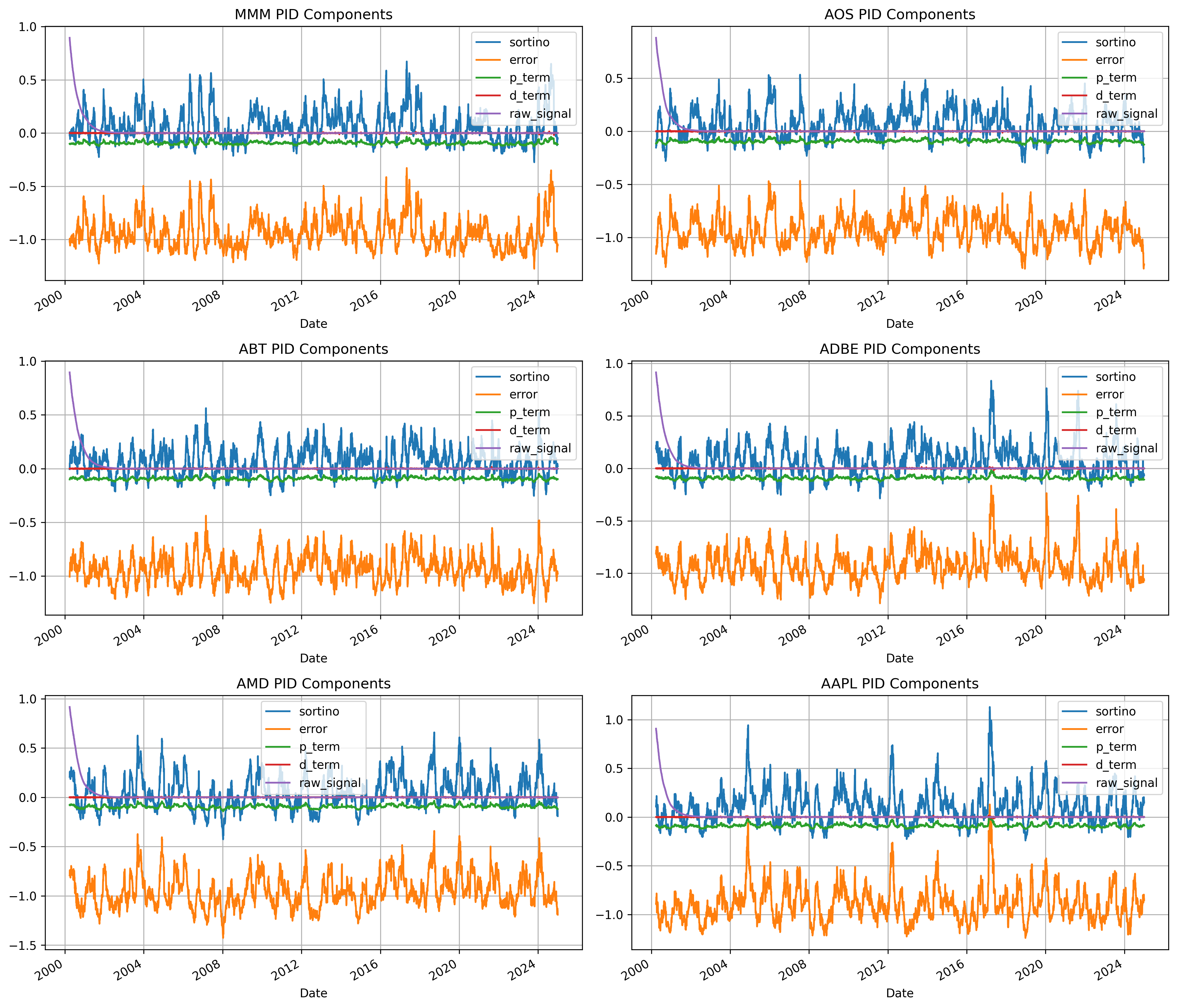
And here’s how some of the assets’s PID controllers look like under the hood.

Getting the Code

Now, you have a fully working and highly profitable weekly rebalancing strategy based on the same principles that govern your thermostat. That’s pretty cool!

If you want to play around with parameters, add your own tickers, etc, go to the private Google Drive to access the entire research notebook to recreate the results.

If you are not a paid subscriber, become one now to unlock this strategy, and every other strategy I have written about on this blog. Every week I post something new, so you’ll never run out of premium content and systems of the highest quantitative analysis quality.

And, like always,

Happy research!