How I Fused Momentum and Mean-Reversion to Achieve 20% CAGR on Liquid Stocks Since 2000

My local adaptive learning system blasted past buy-and-hold.

We think of momentum and mean reversion as opposing forces—pick one or the other. Yet, data from 2000 shows that blending both via a local adaptive learning filter produces 20% CAGR on liquid equities versus 8% buy-and-hold. Traders ignoring this hybrid edge are leaving significant extra returns on the table.

---

In today’s article, I’ll walk you through how I built the LOAD strategy—a clean, single-file Python implementation of Guan & An’s local adaptive learning system—that fuses momentum and mean-reversion into one rotation strategy. The result: a 20% CAGR on liquid equities over the last several decades and ready for your backtester.

Here’s the twist:

Most quants optimize one signal at a time. When you allow your model to adaptively blend both, you unlock hidden return streams that neither strategy could deliver on its own.

Opposing Forces

Momentum and mean reversion are both factors in the market. This means that they both are strategies that have bodies of evidence and research that support their existence and that both of these patterns exist in markets in a profitable way. In fact, both are used by traders in a major way to beat the market.

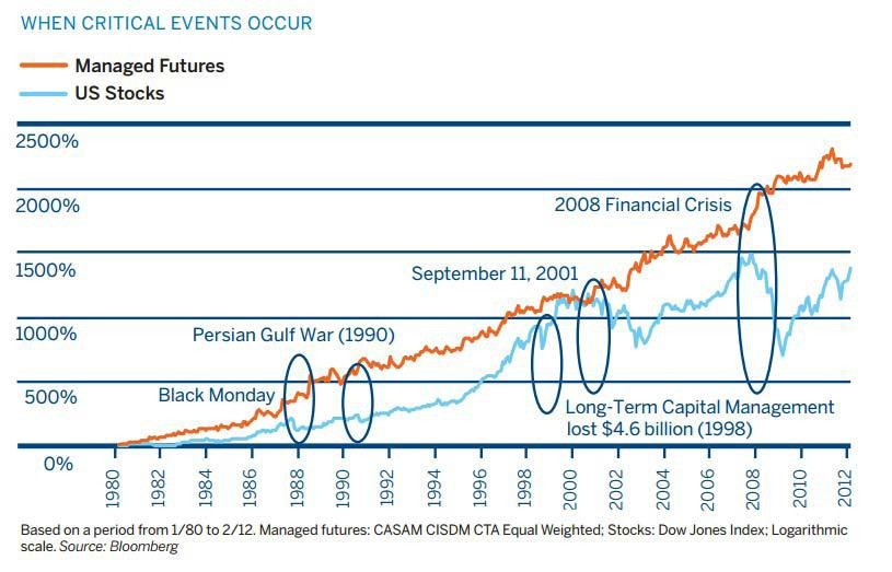
For example, managed futures are strategies employed by CTAs (commodity trading advisors) that regularly outperform the market, as seen below, and only use momentum.

Managed Futures Performance

Money managers calculate which commodities have the best momentum and recent performance and allocate more of their portfolio into those assets.

Buying the Dip

But let’s not forget wall-street’s other favorite strategy, buying the dip. Buy low sell high, right? So you should buy when an asset is low, not when it is performing well.

Illustration of where buying the bottom of a crash would have made you a lot of money, because the SPX is mean reverting and generally bounces back to the trend.

Yet these concepts are diametrically opposed. It’s like black and white. Buying low expecting a bounce is very different than buying a high and expecting it to go higher. But we know that both of these strategies are profitable. How can we reconcile their differences into a single profitable strategy?

Finding the Balance

In Guan and An’s 2019 paper titled: "A local adaptive learning system for online portfolio selection," they attempt to answer this exact question. How do we take advantage of momentum during times of bull runs and mean reversion during times of bear runs?

Their answer is to split an asset’s returns into regimes of ‘bull’ and ‘bear’ where bull markets utilize a momentum strategy and bear utilize a mean-reverting one. To do this, they calculate a simple linear regression on the recent prices to determine a slope. If the slope is positive, we are in a bull market. Otherwise, we are in a bear market.

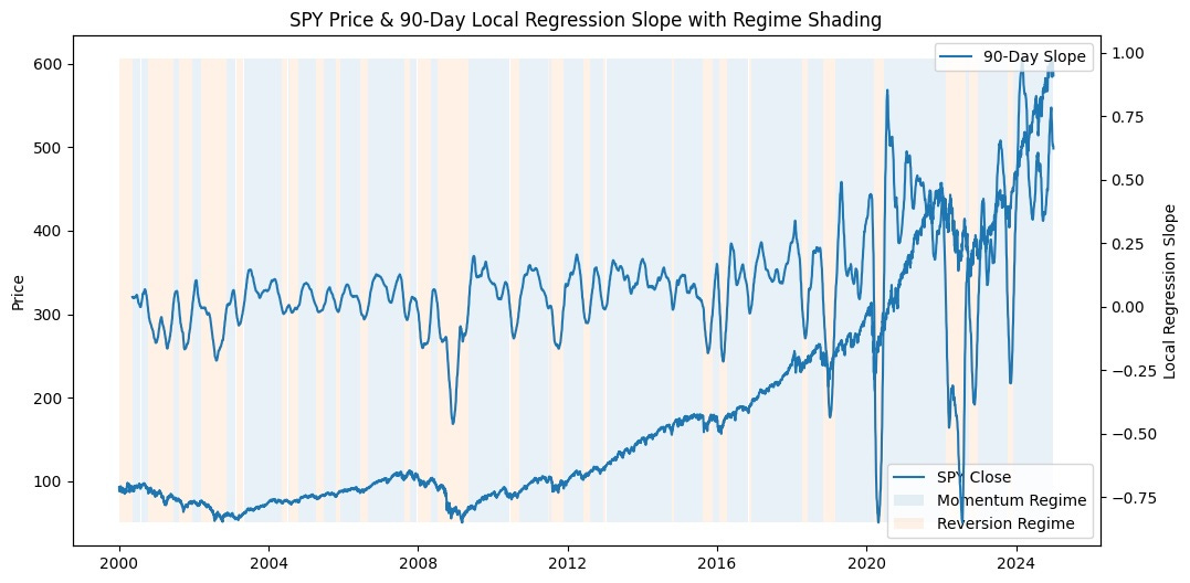
Above is a simple visualization of this concept. When the 90-day local regression slope is positive, we are in a momentum regime. Otherwise, a reversion regime. Visually, you can see how things roughly line up. Downward periods in the SPY line up with reversion regimes and vice versa.

Determining Signal Strength

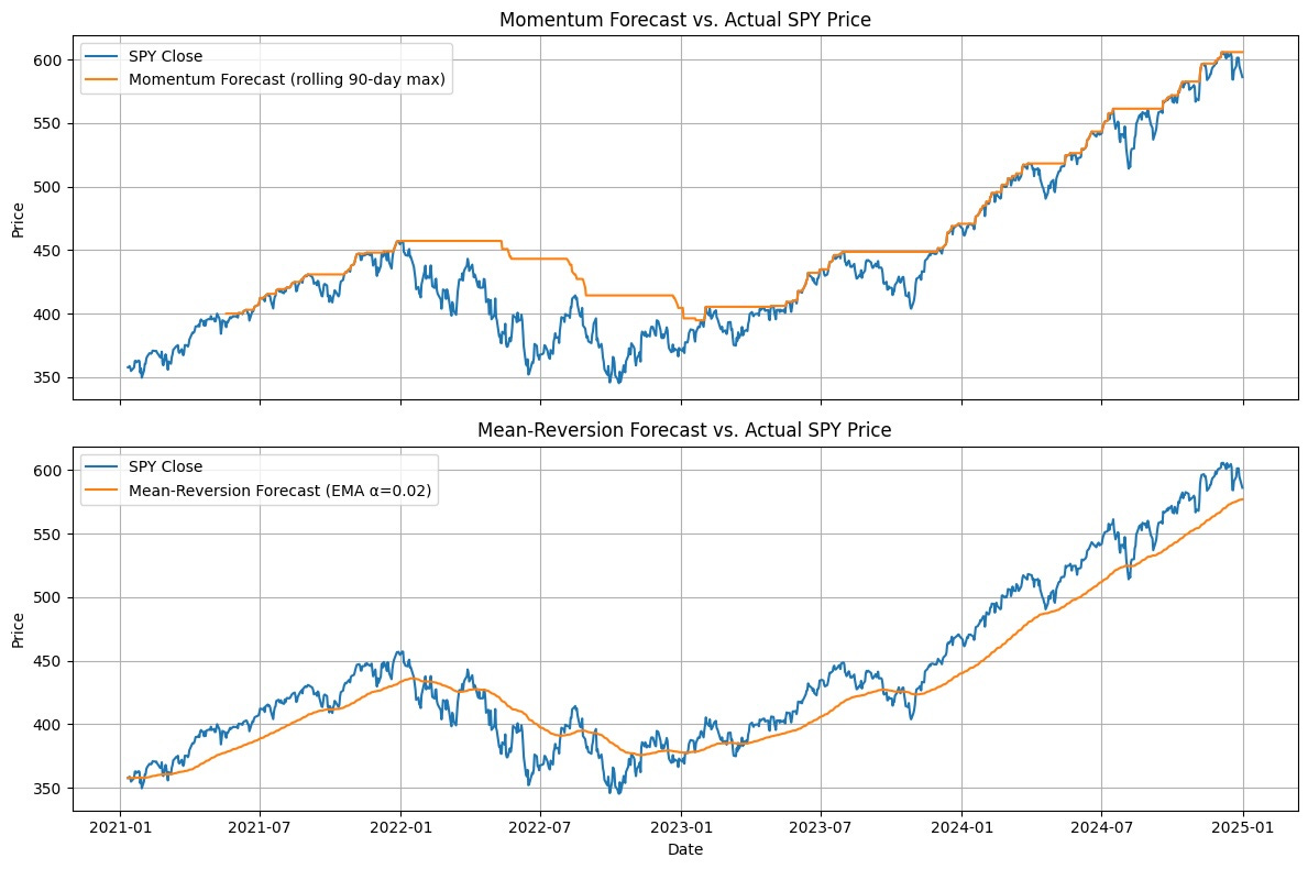
Just because we are in an ‘up’ regime or ‘down’ regime does not mean we are going to magically make money. Guan and An take this into consideration by devising two separate strategies. In the upper chart, you see how during upward periods, the rolling 90-day high continues to climb. The distance between the price and the high is very small. This indicates strength in the regime.

On the contrary, during downward regimes, we expect the price to revert back to the general trend. This trend is calculated with an exponential moving average (EMA). You can see how the price tends to follow the moving average in the bottom chart when the slope of the moving average is negative.

Switching Sides

The LOAD (LOcal ADaptive) system then combines these signals into a single ‘conditional forecast.’ That conditional is based on the regime. Upward regimes look at the rolling high of the asset. Downward regimes look at the moving average. Forecast is a bit of a misnomer, however. It is simply a signal that the system uses to make an investment decision.

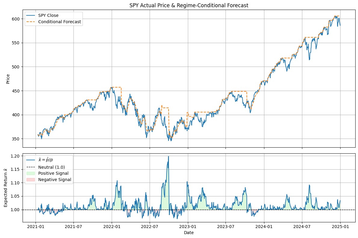
Positive signals are considered buys. Negative signals are considered sells. In other terms, when we have a positive signal (signal > 0), we go long into the asset. Otherwise, we stay in cash. This produces an equity curve like the one below:

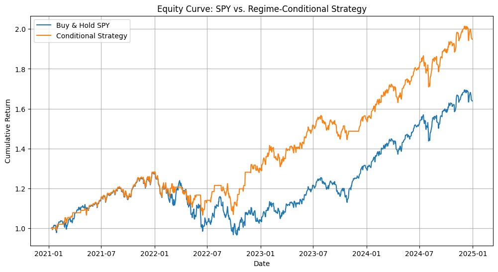
It’s cute. We get a nice edge over the SPY over 4 years. But it’s nothing spectacular. That is, until we start…

Adding the Gasoline

The power of the LOAD system is not in the signals. It’s in the comparative forecasting of each of the signals in a single basket. Whereas the signals produced in our example above show a slight edge, when we rank the signals produced by a basket of assets together and use online-learning to optimize for wealth, we start to really see the power in blending momentum and mean-reversion.

The LOAD system uses something called ‘passive-aggressive’ learning which is a machine learning algorithm (a simple one) that relaxes the system when it is performing well and aggressively learns when new samples (new price data) shows that the current model is wrong.

We start with an equally weighted portfolio and at each step calculate the signals described above. We then have a ‘forecast’ of where we think each asset is headed. We look at our current weights, and what weights would be optimal to satisfy our forecast.

For example, if we have AAPL, MSFT, and META, each weighted at 0.33, 0.33, and 0.33, and our signals show that AAPL and MSFT are going to outperform tomorrow, our optimal weights will be 0.5, 0.5, and 0.

However, for online learning, that ‘jump’ to the new weights is usually not all at once to prevent noisy prices and recent market behavior from destroying our system.

The results? A powerful system that gets over 20% CAGR and is immune to transaction fees.

The Final Results

I used a large basket of high dividend stocks, specifically: ABBV, ABT, AMGN, BMY, CL, CLX, CVS, CVX, GILD, GIS, IBM, JNJ, KHC, KMB, KO, LLY, MCD, MDLZ, MMM, MO, MRK, PEP, PFE, PG, PM, SHY, STZ, T, TLT, VZ, WMT, and XOM. I found that this basket of stocks, with risk-off assets of TLT and SHY performed the best. Have a look for yourself:

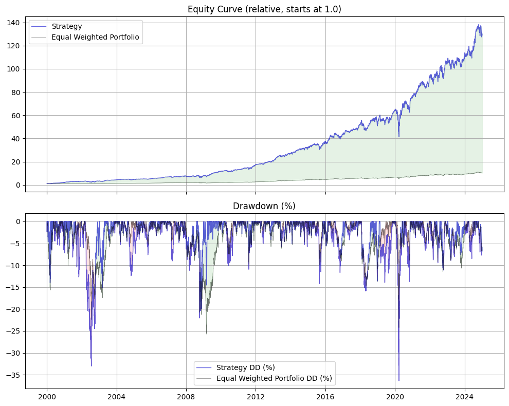
The final figures against the equal weighted portfolio stack up like so:

• Benchmark

  • CAGR: 9.80%

  • Sharpe: 0.74

• LOAD Strategy

  • CAGR: 21.42%

  • Sharpe: 1.16

Transaction Cost Analysis

By using a long window of 180 days to calculate the slope and signals, we avoid a lot of turnover. 10 basis points shaves off about 5% from our CAGR, which is not great, but not terrible. 20 basis points shaves off about 12%, which is still higher than the benchmark and higher than the SPY which gets about 7% CAGR.

Next Steps & How to Get the Code

1. Try It Yourself

   • Grab the full Jupyter notebook, including live data loaders, visualization cells, and the production-ready LOADStrategy implementation.

   • Tweak your own baskets—whether it’s tech, dividends, or global commodities—and see how the system balances them in real time.

2. Join the Inner Circle

   • Paid subscribers get immediate access to the private Google Drive, where you’ll find:

     • The complete guan2019_load.py strategy module for Portwine.

     • Visualizations and analyzers not included for free subscribers that you can use in your own systems.

     • Access to the archives of all strategy code from all previous posts.

Thanks again to all my subscribers, paid or free, and happy researching!